Severn_05: Modeling ungauged stations
Source:vignettes/V05_Modelling_ungauged_nodes.Rmd
V05_Modelling_ungauged_nodes.Rmd
library(airGRiwrm)
#> Loading required package: airGR
#>
#> Attaching package: 'airGRiwrm'
#> The following objects are masked from 'package:airGR':
#>
#>     Calibration, CreateCalibOptions, CreateInputsCrit,
#>     CreateInputsModel, CreateRunOptions, RunModel
An Ungauged station is a virtual hydrometric station where no observed flows are available for calibration.
Why modeling Ungauged station in a semi-distributed model?
Ungauged nodes in a semi-distributed model can be used to reach two different goals:
- increase spatial resolution of the rain fall to improve streamflow simulation (F. Lobligeois et al. 2014).
- simulate streamflows in location of interest for management purpose
This vignette introduces the implementation in airGRiwrm of the method developed by Florent Lobligeois (2014) for calibrating Ungauged nodes in a semi-distributed model.
Presentation of the study case
Using the study case of the vignette #1 and #2, we consider this time
that nodes 54001 and 54029 are
Ungauged. We simulate the streamflow at these locations by
sharing hydrological parameters of the gauged node
54032.
Hydrological parameters at the ungauged nodes will be the same as the
one at the gauged node 54032 except for the unit hydrograph
parameter which depend on the area of the sub-basin. Florent Lobligeois (2014) provides the following
conversion formula for this parameter:
With
the unit hydrograph parameter for the entire basin at 54032
which as an area of
;
the area and
the parameter for the sub-basin
.
Using Ungauged stations in the airGRiwrm model
Ungauged stations are specified by using the model
"Ungauged" in the model column provided in the
CreateGRiwrm function:
data(Severn)
nodes <- Severn$BasinsInfo[, c("gauge_id", "downstream_id", "distance_downstream", "area")]
nodes$model <- "RunModel_GR4J"
nodes$model[nodes$gauge_id %in% c("54029", "54001")] <- "Ungauged"
griwrmV05 <- CreateGRiwrm(
  nodes,
  list(id = "gauge_id", down = "downstream_id", length = "distance_downstream")
)
#> Ungauged node '54001' automatically gets the node '54032' as parameter donor
#> Ungauged node '54029' automatically gets the node '54032' as parameter donor
griwrmV05
#>      id  down length    area         model donor
#> 4 54095 54001     42 3722.68 RunModel_GR4J 54095
#> 5 54002 54057     43 2207.95 RunModel_GR4J 54002
#> 3 54001 54032     45 4329.90      Ungauged 54032
#> 6 54029 54032     32 1483.65      Ungauged 54032
#> 2 54032 54057     15 6864.88 RunModel_GR4J 54032
#> 1 54057  <NA>     NA 9885.46 RunModel_GR4J 54057
It should be noted that the GRiwrm object includes a
column which automatically define the first gauged station at downstream
for each Ungauged node. It is also possible to manually define
the donor node of an Ungauged node, which may be upstream or in
a parallel sub-basin. Type ?CreateGRiwrm for more
details.
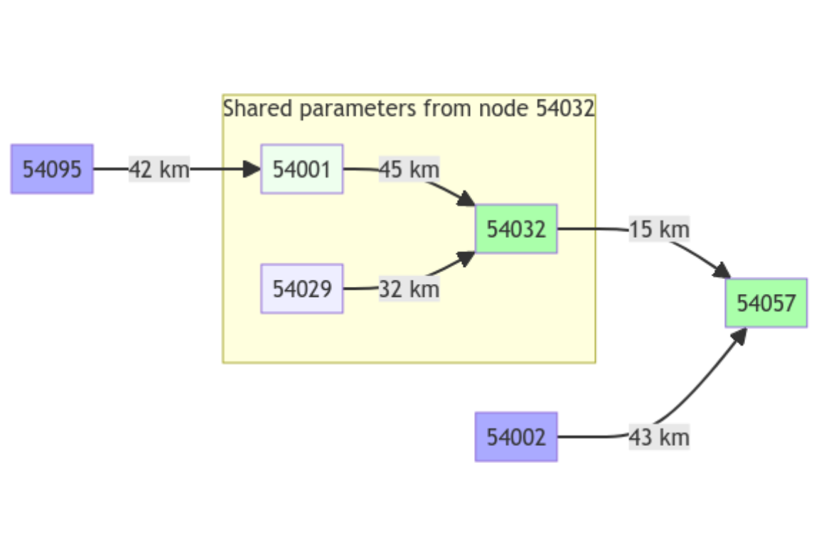
On the following network scheme, the Ungauged nodes are clearer than gauged ones with the same color (blue for upstream nodes and green for intermediate and downstream nodes)
plot(griwrmV05)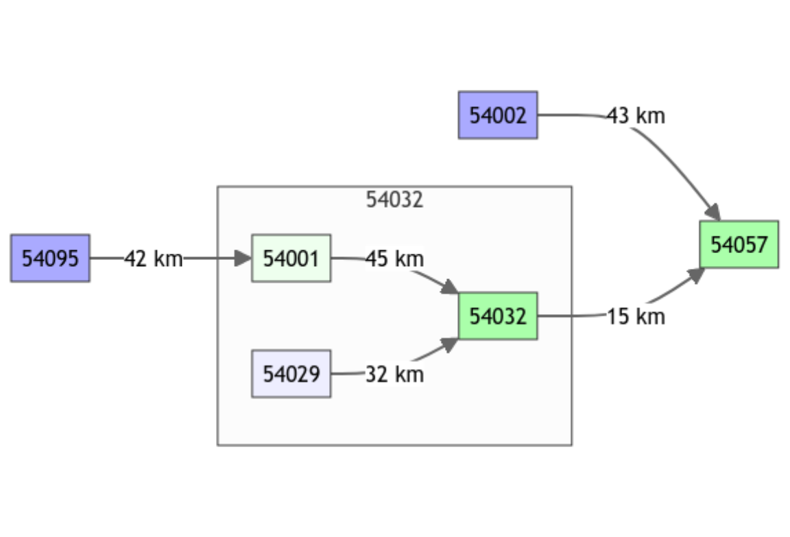
Generation of the GRiwrmInputsModel object
The formatting of the input data is described in the vignette “V01_Structure_SD_model”. The following code chunk resumes this formatting procedure:
BasinsObs <- Severn$BasinsObs
DatesR <- BasinsObs[[1]]$DatesR
PrecipTot <- cbind(sapply(BasinsObs, function(x) {x$precipitation}))
PotEvapTot <- cbind(sapply(BasinsObs, function(x) {x$peti}))
Precip <- ConvertMeteoSD(griwrmV05, PrecipTot)
PotEvap <- ConvertMeteoSD(griwrmV05, PotEvapTot)
Then, the GRiwrmInputsModel object can be generated
taking into account the new GRiwrm object:
IM_U <- CreateInputsModel(griwrmV05, DatesR, Precip, PotEvap)
#> CreateInputsModel.GRiwrm: Processing sub-basin 54095...
#> CreateInputsModel.GRiwrm: Processing sub-basin 54002...
#> CreateInputsModel.GRiwrm: Processing sub-basin 54001...
#> CreateInputsModel.GRiwrm: Processing sub-basin 54029...
#> CreateInputsModel.GRiwrm: Processing sub-basin 54032...
#> CreateInputsModel.GRiwrm: Processing sub-basin 54057...
Calibration of the model integrating ungauged nodes
Calibration options is detailed in vignette “V02_Calibration_SD_model”. We also apply a parameter regularization here but only where an upstream simulated catchment is available.
The following code chunk resumes this procedure:
IndPeriod_Run <- seq(
  which(DatesR == (DatesR[1] + 365*24*60*60)), # Set aside warm-up period
  length(DatesR) # Until the end of the time series
)
IndPeriod_WarmUp = seq(1,IndPeriod_Run[1]-1)
RunOptions <- CreateRunOptions(IM_U,
                               IndPeriod_WarmUp = IndPeriod_WarmUp,
                               IndPeriod_Run = IndPeriod_Run)
Qobs <- cbind(sapply(BasinsObs, function(x) {x$discharge_spec}))
InputsCrit <- CreateInputsCrit(IM_U,
                               FUN_CRIT = ErrorCrit_KGE2,
                               RunOptions = RunOptions, Obs = Qobs[IndPeriod_Run,],
                               AprioriIds = c("54057" = "54032", "54032" = "54095"),
                               transfo = "sqrt", k = 0.15
)
CalibOptions <- CreateCalibOptions(IM_U)
The airGR calibration process is applied on each
hydrological node of the GRiwrm network from upstream nodes
to downstream nodes but this time the calibration of the sub-basin
54032 invokes a semi-distributed model composed of the
nodes 54029, 54001 and 54032
sharing the same parameters.
OC_U <- suppressWarnings(
  Calibration(IM_U, RunOptions, InputsCrit, CalibOptions))
#> Calibration.GRiwrmInputsModel: Processing sub-basin '54095'...
#> Grid-Screening in progress (0% 20% 40% 60% 80% 100%)
#>   Screening completed (81 runs)
#>       Param =  247.151,   -0.020,   83.096,    2.384
#>       Crit. KGE2[sqrt(Q)] = 0.9507
#> Steepest-descent local search in progress
#>   Calibration completed (37 iterations, 377 runs)
#>       Param =  305.633,    0.061,   48.777,    2.733
#>       Crit. KGE2[sqrt(Q)] = 0.9578
#> Calibration.GRiwrmInputsModel: Processing sub-basin '54002'...
#> Grid-Screening in progress (0% 20% 40% 60% 80% 100%)
#>   Screening completed (81 runs)
#>       Param =  432.681,   -0.020,   20.697,    1.944
#>       Crit. KGE2[sqrt(Q)] = 0.9264
#> Steepest-descent local search in progress
#>   Calibration completed (18 iterations, 209 runs)
#>       Param =  389.753,    0.085,   17.870,    2.098
#>       Crit. KGE2[sqrt(Q)] = 0.9370
#> Calibration.GRiwrmInputsModel: Processing sub-basins '54001', '54029', '54032' with '54032' as gauged donor...
#> Parameter regularization: get a priori parameters from node 54095: 1, 305.633, 0.061, 48.777, 1.871
#> Crit. KGE2[sqrt(Q)] = 0.9578
#>  SubCrit. KGE2[sqrt(Q)] cor(sim, obs, "pearson") = 0.9579
#>  SubCrit. KGE2[sqrt(Q)] cv(sim)/cv(obs)          = 1.0023
#>  SubCrit. KGE2[sqrt(Q)] mean(sim)/mean(obs)      = 1.0007
#>
#> Grid-Screening in progress (0% 20% 40% 60% 80% 100%)
#>   Screening completed (243 runs)
#>       Param =    1.250,  432.681,   -0.649,   20.697,    1.944
#>       Crit. Composite    = 0.9624
#> Steepest-descent local search in progress
#>   Calibration completed (23 iterations, 451 runs)
#>       Param =    1.125,  386.196,   -0.611,   31.536,    1.803
#>       Crit. Composite    = 0.9650
#>  Formula: sum(0.86 * KGE2[sqrt(Q)], 0.14 * GAPX[ParamT])
#> Tranferring parameters from node '54032' to node '54001'
#>       Param =    1.125,  386.196,   -0.611,   31.536,    1.529
#>
#> Tranferring parameters from node '54032' to node '54029'
#>       Param =  386.196,   -0.611,   31.536,    1.999
#>
#> Calibration.GRiwrmInputsModel: Processing sub-basin '54057'...
#> Parameter regularization: get a priori parameters from node 54032: 1.125, 386.196, -0.611, 31.536, 1.669
#> Crit. KGE2[sqrt(Q)] = 0.9660
#>  SubCrit. KGE2[sqrt(Q)] cor(sim, obs, "pearson") = 0.9664
#>  SubCrit. KGE2[sqrt(Q)] cv(sim)/cv(obs)          = 1.0013
#>  SubCrit. KGE2[sqrt(Q)] mean(sim)/mean(obs)      = 1.0050
#>
#> Grid-Screening in progress (0% 20% 40% 60% 80% 100%)
#>   Screening completed (243 runs)
#>       Param =    1.250,  432.681,   -0.649,   42.098,    1.944
#>       Crit. Composite    = 0.9609
#> Steepest-descent local search in progress
#>   Calibration completed (23 iterations, 450 runs)
#>       Param =    1.120,  383.753,   -0.613,   31.500,    1.671
#>       Crit. Composite    = 0.9647
#>  Formula: sum(0.85 * KGE2[sqrt(Q)], 0.15 * GAPX[ParamT])
Hydrological parameters for sub-basins
Run the model with the optimized model parameters
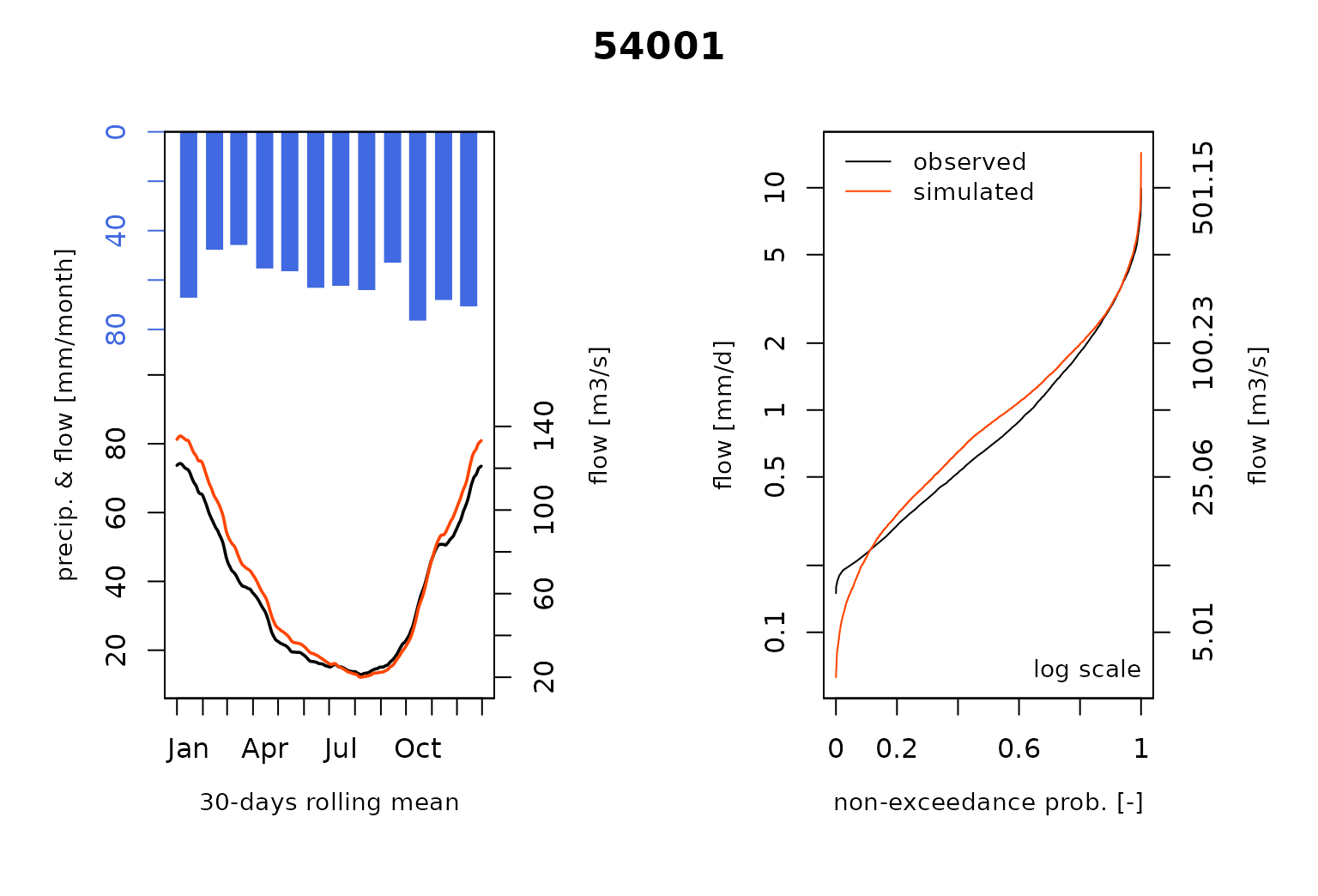
The hydrological model uses parameters inherited from the calibration
of the gauged sub-basin 54032 for the Ungauged
nodes 54001 and 54029:
ParamV05 <- sapply(griwrmV05$id, function(x) {OC_U[[x]]$Param})
dfParam <- do.call(
  rbind,
  lapply(ParamV05, function(x)
    if (length(x)==4) {return(c(NA, x))} else return(x))
)
colnames(dfParam) <- c("velocity", paste0("X", 1:4))
knitr::kable(round(dfParam, 3))| velocity | X1 | X2 | X3 | X4 | |
|---|---|---|---|---|---|
| 54095 | NA | 305.633 | 0.061 | 48.777 | 2.733 |
| 54002 | NA | 389.753 | 0.085 | 17.870 | 2.098 |
| 54001 | 1.125 | 386.196 | -0.611 | 31.536 | 1.529 |
| 54029 | NA | 386.196 | -0.611 | 31.536 | 1.999 |
| 54032 | 1.125 | 386.196 | -0.611 | 31.536 | 1.803 |
| 54057 | 1.120 | 383.753 | -0.613 | 31.500 | 1.671 |
We can run the model with these calibrated parameters:
OutputsModels <- RunModel(
IM_U,
RunOptions = RunOptions,
Param = ParamV05
)
#> RunModel.GRiwrmInputsModel: Processing sub-basin 54095...
#> RunModel.GRiwrmInputsModel: Processing sub-basin 54002...
#> RunModel.GRiwrmInputsModel: Processing sub-basin 54001...
#> RunModel.GRiwrmInputsModel: Processing sub-basin 54029...
#> RunModel.GRiwrmInputsModel: Processing sub-basin 54032...
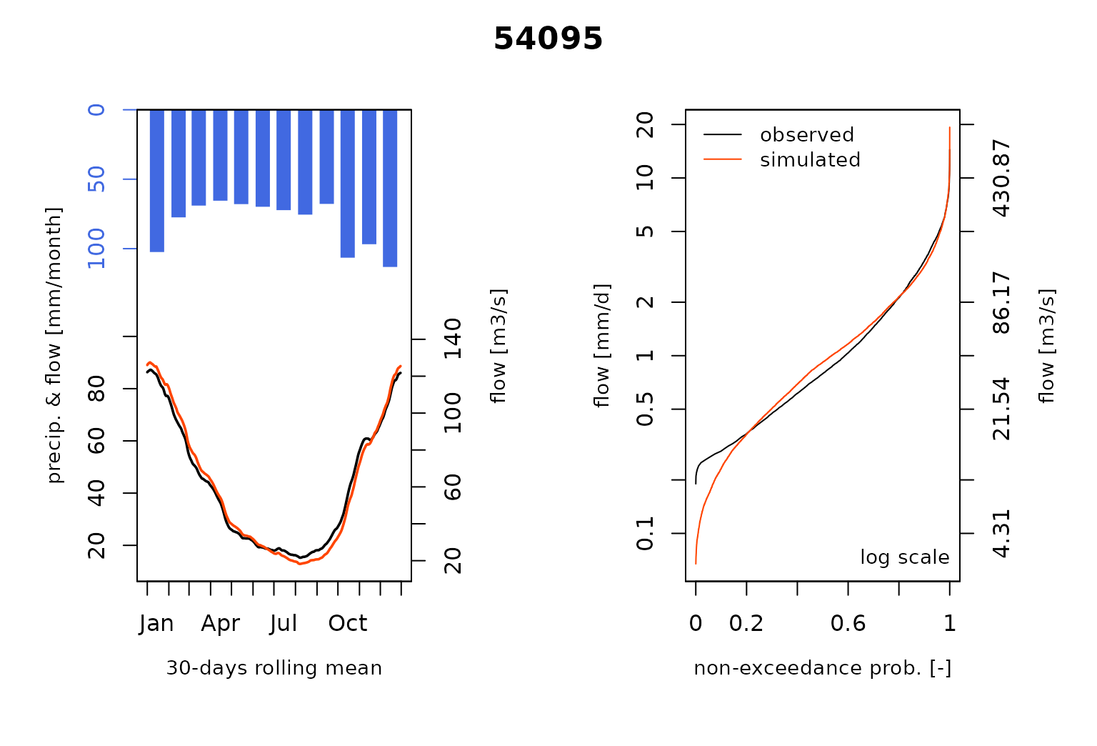
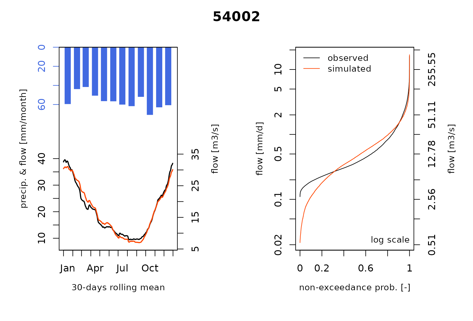
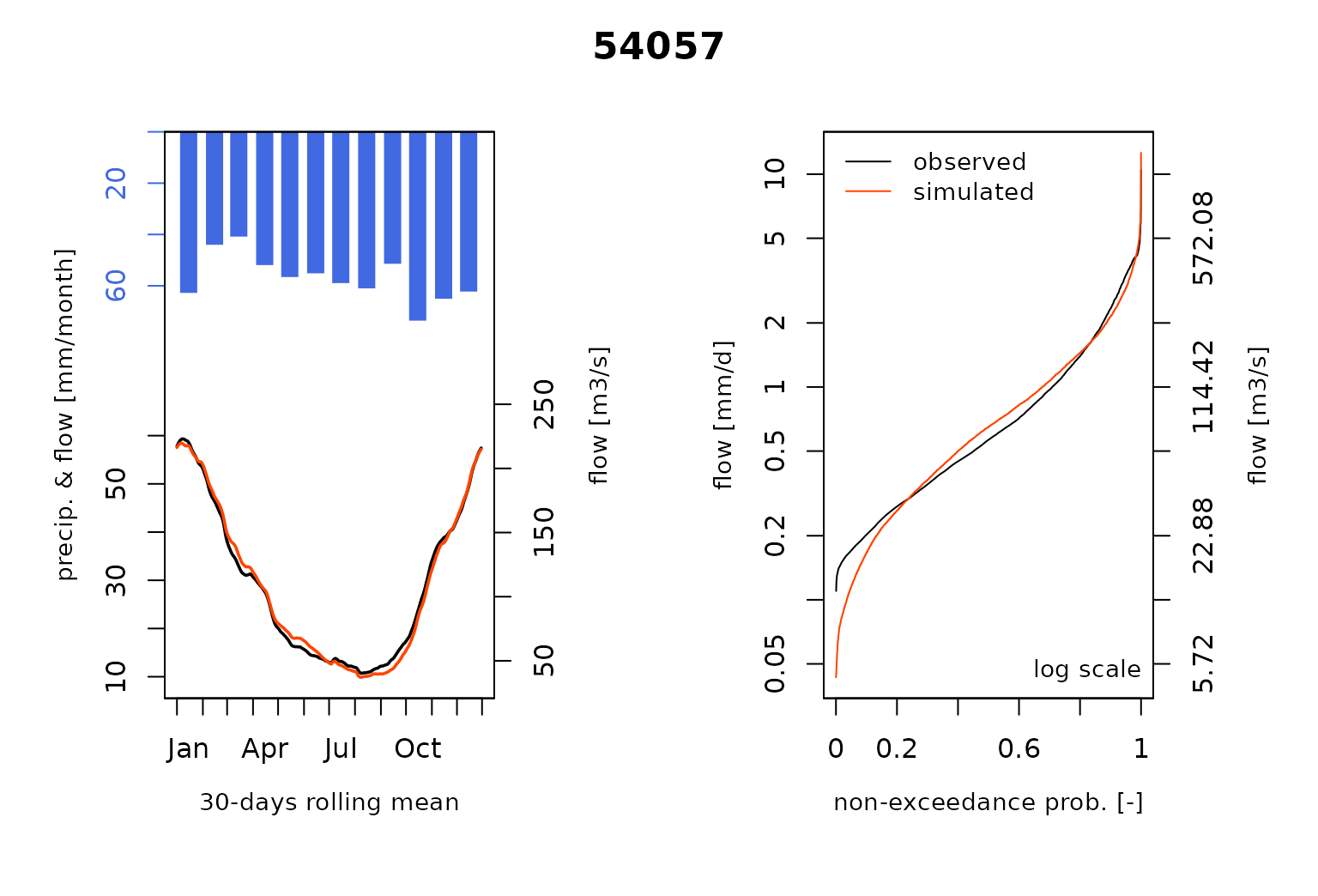
#> RunModel.GRiwrmInputsModel: Processing sub-basin 54057...and plot the comparison of the modeled and the observed flows including the so-called Ungauged stations :