RunModel function for GRiwrmInputsModel object
Source:R/RunModel.GRiwrmInputsModel.R
RunModel.GRiwrmInputsModel.RdRunModel function for GRiwrmInputsModel object
# S3 method for class 'GRiwrmInputsModel'
RunModel(x, RunOptions, Param, ...)
Arguments
- x
[object of class GRiwrmInputsModel] see CreateInputsModel.GRiwrm for details
- RunOptions
[object of class GRiwrmRunOptions] see CreateRunOptions.GRiwrmInputsModel for details
- Param
list parameter values. The list item names are the IDs of the sub-basins. Each item is a numeric vector
- ...
Further arguments for compatibility with S3 methods
Value
An object of class GRiwrmOutputsModel. This object is a list of OutputsModel objects produced by RunModel.InputsModel for each node of the semi-distributed model.
It also contains the following attributes (see attr):
"Qm3s": a data.frame containing the dates of simulation and one column by node with the simulated flows in cubic meters per seconds (See plot.Qm3s)
"GRiwrm": a copy of the GRiwrm object produced by CreateGRiwrm and used for the simulation
"TimeStep": time step of the simulation in seconds
Examples
###################################################################
# Run the `airGR::RunModel_Lag` example in the GRiwrm fashion way #
# Simulation of a reservoir with a purpose of low-flow mitigation #
###################################################################
## ---- preparation of the InputsModel object
## loading package and catchment data
library(airGRiwrm)
data(L0123001)
## ---- specifications of the reservoir
## the reservoir withdraws 1 m3/s when it's possible considering the flow observed in the basin
Qupstream <- matrix(-sapply(BasinObs$Qls / 1000 - 1, function(x) {
min(1, max(0, x, na.rm = TRUE))
}), ncol = 1)
## except between July and September when the reservoir releases 3 m3/s for low-flow mitigation
month <- as.numeric(format(BasinObs$DatesR, "%m"))
Qupstream[month >= 7 & month <= 9] <- 3
Qupstream <- Qupstream * 86400 ## Conversion in m3/day
## the reservoir is not an upstream subcachment: its areas is NA
BasinAreas <- c(NA, BasinInfo$BasinArea)
## delay time between the reservoir and the catchment outlet is 2 days and the distance is 150 km
LengthHydro <- 150
## with a delay of 2 days for 150 km, the flow velocity is 75 km per day
Velocity <- (LengthHydro * 1e3 / 2) / (24 * 60 * 60) ## Conversion km/day -> m/s
# This example is a network of 2 nodes which can be describe like this:
db <- data.frame(id = c("Reservoir", "GaugingDown"),
length = c(LengthHydro, NA),
down = c("GaugingDown", NA),
area = c(NA, BasinInfo$BasinArea),
model = c(NA, "RunModel_GR4J"),
stringsAsFactors = FALSE)
# Create GRiwrm object from the data.frame
griwrm <- CreateGRiwrm(db)
# \dontrun{
plot(griwrm)
 # }
# Formatting observations for the hydrological models
# Each input data should be a matrix or a data.frame with the good id in the name of the column
Precip <- matrix(BasinObs$P, ncol = 1)
colnames(Precip) <- "GaugingDown"
PotEvap <- matrix(BasinObs$E, ncol = 1)
colnames(PotEvap) <- "GaugingDown"
# Observed flows contain flows that are directly injected in the model
Qinf = matrix(Qupstream, ncol = 1)
colnames(Qinf) <- "Reservoir"
# Creation of the GRiwrmInputsModel object (= a named list of InputsModel objects)
InputsModels <- CreateInputsModel(griwrm,
DatesR = BasinObs$DatesR,
Precip = Precip,
PotEvap = PotEvap,
Qinf = Qinf)
#> CreateInputsModel.GRiwrm: Processing sub-basin GaugingDown...
str(InputsModels)
#> List of 1
#> $ GaugingDown:List of 19
#> ..$ DatesR : POSIXlt[1:10593], format: "1984-01-01" "1984-01-02" ...
#> ..$ Precip : num [1:10593] 4.1 15.9 0.8 0 0 0 0 0 2.9 0 ...
#> ..$ PotEvap : num [1:10593] 0.2 0.2 0.3 0.3 0.1 0.3 0.4 0.4 0.5 0.5 ...
#> ..$ Qupstream : num [1:10593, 1] -86400 -86400 -86400 -86400 -86400 -86400 -86400 -86400 -86400 -86400 ...
#> .. ..- attr(*, "dimnames")=List of 2
#> .. .. ..$ : NULL
#> .. .. ..$ : chr "Reservoir"
#> ..$ LengthHydro : Named num 150
#> .. ..- attr(*, "names")= chr "Reservoir"
#> ..$ BasinAreas : Named num [1:2] NA 360
#> .. ..- attr(*, "names")= chr [1:2] "Reservoir" "GaugingDown"
#> ..$ id : chr "GaugingDown"
#> ..$ down : chr NA
#> ..$ UpstreamNodes : chr "Reservoir"
#> ..$ UpstreamIsModeled: Named logi FALSE
#> .. ..- attr(*, "names")= chr "Reservoir"
#> ..$ UpstreamVarQ : Named chr "Qsim_m3"
#> .. ..- attr(*, "names")= chr "Reservoir"
#> ..$ FUN_MOD : chr "RunModel_GR4J"
#> ..$ inUngaugedCluster: logi FALSE
#> ..$ isReceiver : logi FALSE
#> ..$ gaugedId : chr "GaugingDown"
#> ..$ hasUngaugedNodes : logi FALSE
#> ..$ model :List of 4
#> .. ..$ indexParamUngauged: num [1:5] 1 2 3 4 5
#> .. ..$ hasX4 : logi TRUE
#> .. ..$ iX4 : num 5
#> .. ..$ IsHyst : logi FALSE
#> ..$ hasDiversion : logi FALSE
#> ..$ isReservoir : logi FALSE
#> ..- attr(*, "class")= chr [1:5] "RunModel_GR4J" "InputsModel" "daily" "GR" ...
#> - attr(*, "class")= chr [1:2] "GRiwrmInputsModel" "list"
#> - attr(*, "GRiwrm")=Classes ‘GRiwrm’ and 'data.frame': 2 obs. of 6 variables:
#> ..$ id : chr [1:2] "GaugingDown" "Reservoir"
#> ..$ down : chr [1:2] NA "GaugingDown"
#> ..$ length: num [1:2] NA 150
#> ..$ area : num [1:2] 360 NA
#> ..$ model : chr [1:2] "RunModel_GR4J" NA
#> ..$ donor : chr [1:2] "GaugingDown" NA
#> - attr(*, "TimeStep")= num 86400
## run period selection
Ind_Run <- seq(which(format(BasinObs$DatesR, format = "%Y-%m-%d")=="1990-01-01"),
which(format(BasinObs$DatesR, format = "%Y-%m-%d")=="1999-12-31"))
# Creation of the GRiwmRunOptions object
RunOptions <- CreateRunOptions(InputsModels,
IndPeriod_Run = Ind_Run)
#> Warning: model warm up period not defined: default configuration used
#> the year preceding the run period is used
str(RunOptions)
#> List of 1
#> $ GaugingDown:List of 9
#> ..$ IndPeriod_WarmUp: int [1:365] 1828 1829 1830 1831 1832 1833 1834 1835 1836 1837 ...
#> ..$ IndPeriod_Run : int [1:3652] 2193 2194 2195 2196 2197 2198 2199 2200 2201 2202 ...
#> ..$ IniStates : num [1:67] 0 0 0 0 0 0 0 0 0 0 ...
#> ..$ IniResLevels : num [1:4] 0.3 0.5 NA NA
#> ..$ Outputs_Cal : chr [1:2] "Qsim" "Param"
#> ..$ Outputs_Sim : Named chr [1:24] "DatesR" "PotEvap" "Precip" "Prod" ...
#> .. ..- attr(*, "names")= chr [1:24] "" "GR1" "GR2" "GR3" ...
#> ..$ FortranOutputs :List of 2
#> .. ..$ GR: chr [1:18] "PotEvap" "Precip" "Prod" "Pn" ...
#> .. ..$ CN: NULL
#> ..$ FeatFUN_MOD :List of 12
#> .. ..$ CodeMod : chr "GR4J"
#> .. ..$ NameMod : chr "GR4J"
#> .. ..$ NbParam : num 5
#> .. ..$ TimeUnit : chr "daily"
#> .. ..$ Id : logi NA
#> .. ..$ Class : chr [1:2] "daily" "GR"
#> .. ..$ Pkg : chr "airGR"
#> .. ..$ NameFunMod : chr "RunModel_GR4J"
#> .. ..$ TimeStep : num 86400
#> .. ..$ TimeStepMean: int 86400
#> .. ..$ CodeModHydro: chr "GR4J"
#> .. ..$ IsSD : logi TRUE
#> ..$ id : chr "GaugingDown"
#> ..- attr(*, "class")= chr [1:3] "RunOptions" "daily" "GR"
#> - attr(*, "class")= chr [1:2] "list" "GRiwrmRunOptions"
# Parameters of the SD models should be encapsulated in a named list
ParamGR4J <- c(X1 = 257.238, X2 = 1.012, X3 = 88.235, X4 = 2.208)
Param <- list(`GaugingDown` = c(Velocity, ParamGR4J))
# RunModel for the whole network
OutputsModels <- RunModel(InputsModels,
RunOptions = RunOptions,
Param = Param)
#> RunModel.GRiwrmInputsModel: Processing sub-basin GaugingDown...
str(OutputsModels)
#> List of 1
#> $ GaugingDown:List of 24
#> ..$ DatesR : POSIXlt[1:3652], format: "1990-01-01" "1990-01-02" ...
#> ..$ PotEvap : num [1:3652] 0.3 0.4 0.4 0.3 0.1 0.1 0.1 0.2 0.2 0.3 ...
#> ..$ Precip : num [1:3652] 0 9.3 3.2 7.3 0 0 0 0 0.1 0.2 ...
#> ..$ Prod : num [1:3652] 196 199 199 201 200 ...
#> ..$ Pn : num [1:3652] 0 8.9 2.8 7 0 0 0 0 0 0 ...
#> ..$ Ps : num [1:3652] 0 3.65 1.12 2.75 0 ...
#> ..$ AE : num [1:3652] 0.2833 0.4 0.4 0.3 0.0952 ...
#> ..$ Perc : num [1:3652] 0.645 0.696 0.703 0.74 0.725 ...
#> ..$ PR : num [1:3652] 0.645 5.946 2.383 4.992 0.725 ...
#> ..$ Q9 : num [1:3652] 1.78 1.52 3.86 3.17 3.45 ...
#> ..$ Q1 : num [1:3652] 0.2 0.195 0.271 0.387 0.365 ...
#> ..$ Rout : num [1:3652] 53.9 53.6 55.3 56.1 56.9 ...
#> ..$ Exch : num [1:3652] 0.181 0.18 0.176 0.197 0.207 ...
#> ..$ AExch1 : num [1:3652] 0.181 0.18 0.176 0.197 0.207 ...
#> ..$ AExch2 : num [1:3652] 0.181 0.18 0.176 0.197 0.207 ...
#> ..$ AExch : num [1:3652] 0.362 0.36 0.353 0.393 0.414 ...
#> ..$ QR : num [1:3652] 2.05 1.99 2.36 2.55 2.78 ...
#> ..$ QD : num [1:3652] 0.381 0.375 0.447 0.584 0.572 ...
#> ..$ Qsim : num [1:3652] 2.43 2.37 2.56 2.9 3.11 ...
#> ..$ RunOptions:List of 4
#> .. ..$ WarmUpQsim : num [1:365] 0.539 0.575 0.807 0.731 0.674 ...
#> .. ..$ Param : Named num [1:5] 0.868 257.238 1.012 88.235 2.208
#> .. .. ..- attr(*, "names")= chr [1:5] "" "" "" "" ...
#> .. ..$ TimeStep : num 86400
#> .. ..$ WarmUpQsim_m3: num [1:365] 194033 206850 290390 263330 242814 ...
#> ..$ StateEnd :List of 4
#> .. ..$ Store :List of 4
#> .. .. ..$ Prod: num 189
#> .. .. ..$ Rout: num 48.9
#> .. .. ..$ Exp : num NA
#> .. .. ..$ Int : num NA
#> .. ..$ UH :List of 2
#> .. .. ..$ UH1: num [1:20] 0.514 0.54 0.148 0 0 ...
#> .. .. ..$ UH2: num [1:40] 0.056306 0.057176 0.042254 0.012188 0.000578 ...
#> .. ..$ CemaNeigeLayers:List of 4
#> .. .. ..$ G : num NA
#> .. .. ..$ eTG : num NA
#> .. .. ..$ Gthr : num NA
#> .. .. ..$ Glocmax: num NA
#> .. ..$ SD :List of 1
#> .. .. ..$ : num [1:3] -86400 -86400 -86400
#> .. ..- attr(*, "class")= chr [1:3] "IniStates" "daily" "GR"
#> ..$ Qsim_m3 : num [1:3652] 875333 851839 922461 1042434 1119947 ...
#> ..$ QsimDown : num [1:3652] 2.43 2.37 2.8 3.14 3.35 ...
#> ..$ Qover_m3 : num [1:3652] 0 0 0 0 0 0 0 0 0 0 ...
#> ..- attr(*, "class")= chr [1:4] "OutputsModel" "daily" "GR" "SD"
#> - attr(*, "class")= chr [1:2] "GRiwrmOutputsModel" "list"
#> - attr(*, "Qm3s")=Classes ‘Qm3s’ and 'data.frame': 3652 obs. of 3 variables:
#> ..$ DatesR : POSIXct[1:3652], format: "1990-01-01" "1990-01-02" ...
#> ..$ GaugingDown: num [1:3652] 10.13 9.86 10.68 12.07 12.96 ...
#> ..$ Reservoir : num [1:3652] -1 -1 -1 -1 -1 -1 -1 -1 -1 -1 ...
#> - attr(*, "GRiwrm")=Classes ‘GRiwrm’ and 'data.frame': 2 obs. of 6 variables:
#> ..$ id : chr [1:2] "GaugingDown" "Reservoir"
#> ..$ down : chr [1:2] NA "GaugingDown"
#> ..$ length: num [1:2] NA 150
#> ..$ area : num [1:2] 360 NA
#> ..$ model : chr [1:2] "RunModel_GR4J" NA
#> ..$ donor : chr [1:2] "GaugingDown" NA
#> - attr(*, "TimeStep")= num 86400
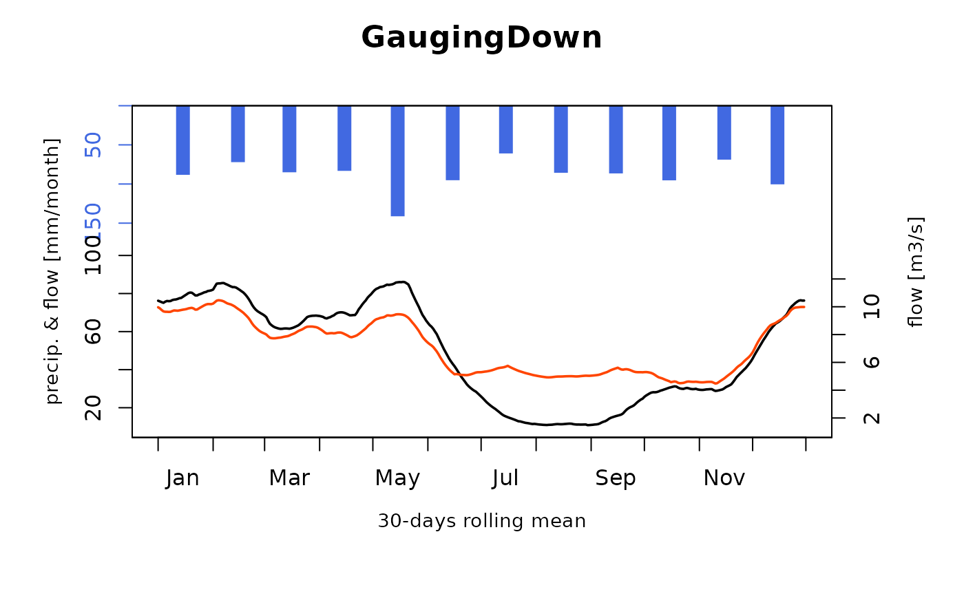
# Compare regimes of the simulation with reservoir and observation of natural flow
plot(OutputsModels,
data.frame(GaugingDown = BasinObs$Qmm[Ind_Run]),
which = "Regime")
# }
# Formatting observations for the hydrological models
# Each input data should be a matrix or a data.frame with the good id in the name of the column
Precip <- matrix(BasinObs$P, ncol = 1)
colnames(Precip) <- "GaugingDown"
PotEvap <- matrix(BasinObs$E, ncol = 1)
colnames(PotEvap) <- "GaugingDown"
# Observed flows contain flows that are directly injected in the model
Qinf = matrix(Qupstream, ncol = 1)
colnames(Qinf) <- "Reservoir"
# Creation of the GRiwrmInputsModel object (= a named list of InputsModel objects)
InputsModels <- CreateInputsModel(griwrm,
DatesR = BasinObs$DatesR,
Precip = Precip,
PotEvap = PotEvap,
Qinf = Qinf)
#> CreateInputsModel.GRiwrm: Processing sub-basin GaugingDown...
str(InputsModels)
#> List of 1
#> $ GaugingDown:List of 19
#> ..$ DatesR : POSIXlt[1:10593], format: "1984-01-01" "1984-01-02" ...
#> ..$ Precip : num [1:10593] 4.1 15.9 0.8 0 0 0 0 0 2.9 0 ...
#> ..$ PotEvap : num [1:10593] 0.2 0.2 0.3 0.3 0.1 0.3 0.4 0.4 0.5 0.5 ...
#> ..$ Qupstream : num [1:10593, 1] -86400 -86400 -86400 -86400 -86400 -86400 -86400 -86400 -86400 -86400 ...
#> .. ..- attr(*, "dimnames")=List of 2
#> .. .. ..$ : NULL
#> .. .. ..$ : chr "Reservoir"
#> ..$ LengthHydro : Named num 150
#> .. ..- attr(*, "names")= chr "Reservoir"
#> ..$ BasinAreas : Named num [1:2] NA 360
#> .. ..- attr(*, "names")= chr [1:2] "Reservoir" "GaugingDown"
#> ..$ id : chr "GaugingDown"
#> ..$ down : chr NA
#> ..$ UpstreamNodes : chr "Reservoir"
#> ..$ UpstreamIsModeled: Named logi FALSE
#> .. ..- attr(*, "names")= chr "Reservoir"
#> ..$ UpstreamVarQ : Named chr "Qsim_m3"
#> .. ..- attr(*, "names")= chr "Reservoir"
#> ..$ FUN_MOD : chr "RunModel_GR4J"
#> ..$ inUngaugedCluster: logi FALSE
#> ..$ isReceiver : logi FALSE
#> ..$ gaugedId : chr "GaugingDown"
#> ..$ hasUngaugedNodes : logi FALSE
#> ..$ model :List of 4
#> .. ..$ indexParamUngauged: num [1:5] 1 2 3 4 5
#> .. ..$ hasX4 : logi TRUE
#> .. ..$ iX4 : num 5
#> .. ..$ IsHyst : logi FALSE
#> ..$ hasDiversion : logi FALSE
#> ..$ isReservoir : logi FALSE
#> ..- attr(*, "class")= chr [1:5] "RunModel_GR4J" "InputsModel" "daily" "GR" ...
#> - attr(*, "class")= chr [1:2] "GRiwrmInputsModel" "list"
#> - attr(*, "GRiwrm")=Classes ‘GRiwrm’ and 'data.frame': 2 obs. of 6 variables:
#> ..$ id : chr [1:2] "GaugingDown" "Reservoir"
#> ..$ down : chr [1:2] NA "GaugingDown"
#> ..$ length: num [1:2] NA 150
#> ..$ area : num [1:2] 360 NA
#> ..$ model : chr [1:2] "RunModel_GR4J" NA
#> ..$ donor : chr [1:2] "GaugingDown" NA
#> - attr(*, "TimeStep")= num 86400
## run period selection
Ind_Run <- seq(which(format(BasinObs$DatesR, format = "%Y-%m-%d")=="1990-01-01"),
which(format(BasinObs$DatesR, format = "%Y-%m-%d")=="1999-12-31"))
# Creation of the GRiwmRunOptions object
RunOptions <- CreateRunOptions(InputsModels,
IndPeriod_Run = Ind_Run)
#> Warning: model warm up period not defined: default configuration used
#> the year preceding the run period is used
str(RunOptions)
#> List of 1
#> $ GaugingDown:List of 9
#> ..$ IndPeriod_WarmUp: int [1:365] 1828 1829 1830 1831 1832 1833 1834 1835 1836 1837 ...
#> ..$ IndPeriod_Run : int [1:3652] 2193 2194 2195 2196 2197 2198 2199 2200 2201 2202 ...
#> ..$ IniStates : num [1:67] 0 0 0 0 0 0 0 0 0 0 ...
#> ..$ IniResLevels : num [1:4] 0.3 0.5 NA NA
#> ..$ Outputs_Cal : chr [1:2] "Qsim" "Param"
#> ..$ Outputs_Sim : Named chr [1:24] "DatesR" "PotEvap" "Precip" "Prod" ...
#> .. ..- attr(*, "names")= chr [1:24] "" "GR1" "GR2" "GR3" ...
#> ..$ FortranOutputs :List of 2
#> .. ..$ GR: chr [1:18] "PotEvap" "Precip" "Prod" "Pn" ...
#> .. ..$ CN: NULL
#> ..$ FeatFUN_MOD :List of 12
#> .. ..$ CodeMod : chr "GR4J"
#> .. ..$ NameMod : chr "GR4J"
#> .. ..$ NbParam : num 5
#> .. ..$ TimeUnit : chr "daily"
#> .. ..$ Id : logi NA
#> .. ..$ Class : chr [1:2] "daily" "GR"
#> .. ..$ Pkg : chr "airGR"
#> .. ..$ NameFunMod : chr "RunModel_GR4J"
#> .. ..$ TimeStep : num 86400
#> .. ..$ TimeStepMean: int 86400
#> .. ..$ CodeModHydro: chr "GR4J"
#> .. ..$ IsSD : logi TRUE
#> ..$ id : chr "GaugingDown"
#> ..- attr(*, "class")= chr [1:3] "RunOptions" "daily" "GR"
#> - attr(*, "class")= chr [1:2] "list" "GRiwrmRunOptions"
# Parameters of the SD models should be encapsulated in a named list
ParamGR4J <- c(X1 = 257.238, X2 = 1.012, X3 = 88.235, X4 = 2.208)
Param <- list(`GaugingDown` = c(Velocity, ParamGR4J))
# RunModel for the whole network
OutputsModels <- RunModel(InputsModels,
RunOptions = RunOptions,
Param = Param)
#> RunModel.GRiwrmInputsModel: Processing sub-basin GaugingDown...
str(OutputsModels)
#> List of 1
#> $ GaugingDown:List of 24
#> ..$ DatesR : POSIXlt[1:3652], format: "1990-01-01" "1990-01-02" ...
#> ..$ PotEvap : num [1:3652] 0.3 0.4 0.4 0.3 0.1 0.1 0.1 0.2 0.2 0.3 ...
#> ..$ Precip : num [1:3652] 0 9.3 3.2 7.3 0 0 0 0 0.1 0.2 ...
#> ..$ Prod : num [1:3652] 196 199 199 201 200 ...
#> ..$ Pn : num [1:3652] 0 8.9 2.8 7 0 0 0 0 0 0 ...
#> ..$ Ps : num [1:3652] 0 3.65 1.12 2.75 0 ...
#> ..$ AE : num [1:3652] 0.2833 0.4 0.4 0.3 0.0952 ...
#> ..$ Perc : num [1:3652] 0.645 0.696 0.703 0.74 0.725 ...
#> ..$ PR : num [1:3652] 0.645 5.946 2.383 4.992 0.725 ...
#> ..$ Q9 : num [1:3652] 1.78 1.52 3.86 3.17 3.45 ...
#> ..$ Q1 : num [1:3652] 0.2 0.195 0.271 0.387 0.365 ...
#> ..$ Rout : num [1:3652] 53.9 53.6 55.3 56.1 56.9 ...
#> ..$ Exch : num [1:3652] 0.181 0.18 0.176 0.197 0.207 ...
#> ..$ AExch1 : num [1:3652] 0.181 0.18 0.176 0.197 0.207 ...
#> ..$ AExch2 : num [1:3652] 0.181 0.18 0.176 0.197 0.207 ...
#> ..$ AExch : num [1:3652] 0.362 0.36 0.353 0.393 0.414 ...
#> ..$ QR : num [1:3652] 2.05 1.99 2.36 2.55 2.78 ...
#> ..$ QD : num [1:3652] 0.381 0.375 0.447 0.584 0.572 ...
#> ..$ Qsim : num [1:3652] 2.43 2.37 2.56 2.9 3.11 ...
#> ..$ RunOptions:List of 4
#> .. ..$ WarmUpQsim : num [1:365] 0.539 0.575 0.807 0.731 0.674 ...
#> .. ..$ Param : Named num [1:5] 0.868 257.238 1.012 88.235 2.208
#> .. .. ..- attr(*, "names")= chr [1:5] "" "" "" "" ...
#> .. ..$ TimeStep : num 86400
#> .. ..$ WarmUpQsim_m3: num [1:365] 194033 206850 290390 263330 242814 ...
#> ..$ StateEnd :List of 4
#> .. ..$ Store :List of 4
#> .. .. ..$ Prod: num 189
#> .. .. ..$ Rout: num 48.9
#> .. .. ..$ Exp : num NA
#> .. .. ..$ Int : num NA
#> .. ..$ UH :List of 2
#> .. .. ..$ UH1: num [1:20] 0.514 0.54 0.148 0 0 ...
#> .. .. ..$ UH2: num [1:40] 0.056306 0.057176 0.042254 0.012188 0.000578 ...
#> .. ..$ CemaNeigeLayers:List of 4
#> .. .. ..$ G : num NA
#> .. .. ..$ eTG : num NA
#> .. .. ..$ Gthr : num NA
#> .. .. ..$ Glocmax: num NA
#> .. ..$ SD :List of 1
#> .. .. ..$ : num [1:3] -86400 -86400 -86400
#> .. ..- attr(*, "class")= chr [1:3] "IniStates" "daily" "GR"
#> ..$ Qsim_m3 : num [1:3652] 875333 851839 922461 1042434 1119947 ...
#> ..$ QsimDown : num [1:3652] 2.43 2.37 2.8 3.14 3.35 ...
#> ..$ Qover_m3 : num [1:3652] 0 0 0 0 0 0 0 0 0 0 ...
#> ..- attr(*, "class")= chr [1:4] "OutputsModel" "daily" "GR" "SD"
#> - attr(*, "class")= chr [1:2] "GRiwrmOutputsModel" "list"
#> - attr(*, "Qm3s")=Classes ‘Qm3s’ and 'data.frame': 3652 obs. of 3 variables:
#> ..$ DatesR : POSIXct[1:3652], format: "1990-01-01" "1990-01-02" ...
#> ..$ GaugingDown: num [1:3652] 10.13 9.86 10.68 12.07 12.96 ...
#> ..$ Reservoir : num [1:3652] -1 -1 -1 -1 -1 -1 -1 -1 -1 -1 ...
#> - attr(*, "GRiwrm")=Classes ‘GRiwrm’ and 'data.frame': 2 obs. of 6 variables:
#> ..$ id : chr [1:2] "GaugingDown" "Reservoir"
#> ..$ down : chr [1:2] NA "GaugingDown"
#> ..$ length: num [1:2] NA 150
#> ..$ area : num [1:2] 360 NA
#> ..$ model : chr [1:2] "RunModel_GR4J" NA
#> ..$ donor : chr [1:2] "GaugingDown" NA
#> - attr(*, "TimeStep")= num 86400
# Compare regimes of the simulation with reservoir and observation of natural flow
plot(OutputsModels,
data.frame(GaugingDown = BasinObs$Qmm[Ind_Run]),
which = "Regime")
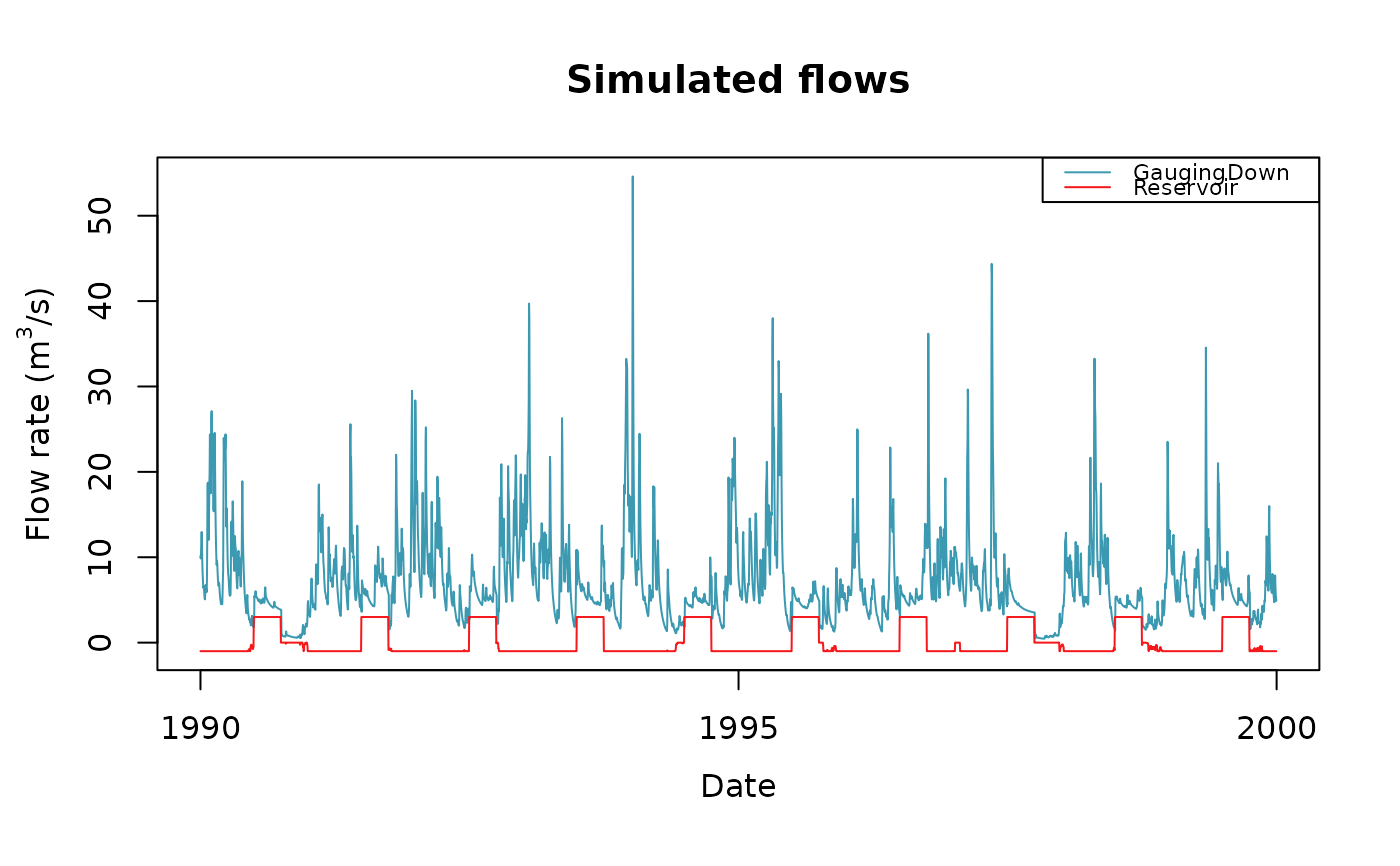 # Plot together simulated flows (m3/s) of the reservoir and the gauging station
plot(attr(OutputsModels, "Qm3s"))
# Plot together simulated flows (m3/s) of the reservoir and the gauging station
plot(attr(OutputsModels, "Qm3s"))
 ########################################################
# Run the Severn example provided with this package #
# A natural catchment composed with 6 gauging stations #
########################################################
data(Severn)
nodes <- Severn$BasinsInfo
nodes$model <- "RunModel_GR4J"
# Mismatch column names are renamed to stick with GRiwrm requirements
rename_columns <- list(id = "gauge_id",
down = "downstream_id",
length = "distance_downstream")
g_severn <- CreateGRiwrm(nodes, rename_columns)
# Network diagram with upstream basin nodes in blue, intermediate sub-basin in green
# \dontrun{
plot(g_severn)
########################################################
# Run the Severn example provided with this package #
# A natural catchment composed with 6 gauging stations #
########################################################
data(Severn)
nodes <- Severn$BasinsInfo
nodes$model <- "RunModel_GR4J"
# Mismatch column names are renamed to stick with GRiwrm requirements
rename_columns <- list(id = "gauge_id",
down = "downstream_id",
length = "distance_downstream")
g_severn <- CreateGRiwrm(nodes, rename_columns)
# Network diagram with upstream basin nodes in blue, intermediate sub-basin in green
# \dontrun{
plot(g_severn)
 # }
# Format CAMEL-GB meteorological dataset for airGRiwrm inputs
BasinsObs <- Severn$BasinsObs
DatesR <- BasinsObs[[1]]$DatesR
PrecipTot <- cbind(sapply(BasinsObs, function(x) {x$precipitation}))
PotEvapTot <- cbind(sapply(BasinsObs, function(x) {x$peti}))
# Precipitation and Potential Evaporation are related to the whole catchment
# at each gauging station. We need to compute them for intermediate catchments
# for use in a semi-distributed model
Precip <- ConvertMeteoSD(g_severn, PrecipTot)
PotEvap <- ConvertMeteoSD(g_severn, PotEvapTot)
# CreateInputsModel object
IM_severn <- CreateInputsModel(g_severn, DatesR, Precip, PotEvap)
#> CreateInputsModel.GRiwrm: Processing sub-basin 54095...
#> CreateInputsModel.GRiwrm: Processing sub-basin 54002...
#> CreateInputsModel.GRiwrm: Processing sub-basin 54029...
#> CreateInputsModel.GRiwrm: Processing sub-basin 54001...
#> CreateInputsModel.GRiwrm: Processing sub-basin 54032...
#> CreateInputsModel.GRiwrm: Processing sub-basin 54057...
# GRiwrmRunOptions object
# Run period is set aside the one-year warm-up period
IndPeriod_Run <- seq(
which(IM_severn[[1]]$DatesR == (IM_severn[[1]]$DatesR[1] + 365*24*60*60)),
length(IM_severn[[1]]$DatesR) # Until the end of the time series
)
IndPeriod_WarmUp <- seq(1, IndPeriod_Run[1] - 1)
RO_severn <- CreateRunOptions(
IM_severn,
IndPeriod_WarmUp = IndPeriod_WarmUp,
IndPeriod_Run = IndPeriod_Run
)
# Load parameters of the model from Calibration in vignette V02
P_severn <- readRDS(system.file("vignettes", "ParamV02.RDS", package = "airGRiwrm"))
# Run the simulation
OM_severn <- RunModel(IM_severn,
RunOptions = RO_severn,
Param = P_severn)
#> RunModel.GRiwrmInputsModel: Processing sub-basin 54095...
#> RunModel.GRiwrmInputsModel: Processing sub-basin 54002...
#> RunModel.GRiwrmInputsModel: Processing sub-basin 54029...
#> RunModel.GRiwrmInputsModel: Processing sub-basin 54001...
#> RunModel.GRiwrmInputsModel: Processing sub-basin 54032...
#> RunModel.GRiwrmInputsModel: Processing sub-basin 54057...
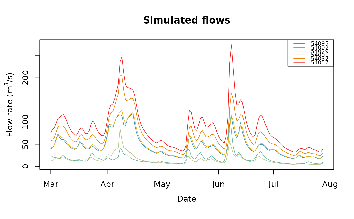
# Plot results of simulated flows in m3/s
Qm3s <- attr(OM_severn, "Qm3s")
plot(Qm3s[1:150, ])
# }
# Format CAMEL-GB meteorological dataset for airGRiwrm inputs
BasinsObs <- Severn$BasinsObs
DatesR <- BasinsObs[[1]]$DatesR
PrecipTot <- cbind(sapply(BasinsObs, function(x) {x$precipitation}))
PotEvapTot <- cbind(sapply(BasinsObs, function(x) {x$peti}))
# Precipitation and Potential Evaporation are related to the whole catchment
# at each gauging station. We need to compute them for intermediate catchments
# for use in a semi-distributed model
Precip <- ConvertMeteoSD(g_severn, PrecipTot)
PotEvap <- ConvertMeteoSD(g_severn, PotEvapTot)
# CreateInputsModel object
IM_severn <- CreateInputsModel(g_severn, DatesR, Precip, PotEvap)
#> CreateInputsModel.GRiwrm: Processing sub-basin 54095...
#> CreateInputsModel.GRiwrm: Processing sub-basin 54002...
#> CreateInputsModel.GRiwrm: Processing sub-basin 54029...
#> CreateInputsModel.GRiwrm: Processing sub-basin 54001...
#> CreateInputsModel.GRiwrm: Processing sub-basin 54032...
#> CreateInputsModel.GRiwrm: Processing sub-basin 54057...
# GRiwrmRunOptions object
# Run period is set aside the one-year warm-up period
IndPeriod_Run <- seq(
which(IM_severn[[1]]$DatesR == (IM_severn[[1]]$DatesR[1] + 365*24*60*60)),
length(IM_severn[[1]]$DatesR) # Until the end of the time series
)
IndPeriod_WarmUp <- seq(1, IndPeriod_Run[1] - 1)
RO_severn <- CreateRunOptions(
IM_severn,
IndPeriod_WarmUp = IndPeriod_WarmUp,
IndPeriod_Run = IndPeriod_Run
)
# Load parameters of the model from Calibration in vignette V02
P_severn <- readRDS(system.file("vignettes", "ParamV02.RDS", package = "airGRiwrm"))
# Run the simulation
OM_severn <- RunModel(IM_severn,
RunOptions = RO_severn,
Param = P_severn)
#> RunModel.GRiwrmInputsModel: Processing sub-basin 54095...
#> RunModel.GRiwrmInputsModel: Processing sub-basin 54002...
#> RunModel.GRiwrmInputsModel: Processing sub-basin 54029...
#> RunModel.GRiwrmInputsModel: Processing sub-basin 54001...
#> RunModel.GRiwrmInputsModel: Processing sub-basin 54032...
#> RunModel.GRiwrmInputsModel: Processing sub-basin 54057...
# Plot results of simulated flows in m3/s
Qm3s <- attr(OM_severn, "Qm3s")
plot(Qm3s[1:150, ])
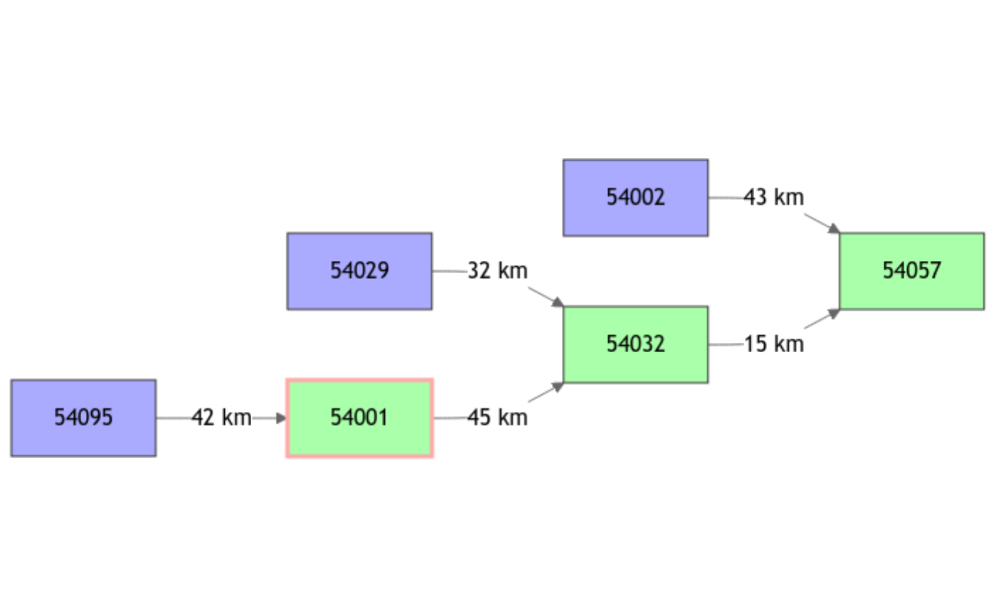
 ##################################################################
# An example of water withdrawal for irrigation with restriction #
# modeled with a Diversion node on the Severn river #
##################################################################
# A diversion is added at gauging station "54001"
nodes_div <- nodes[, c("gauge_id", "downstream_id", "distance_downstream", "area", "model")]
names(nodes_div) <- c("id", "down", "length", "area", "model")
nodes_div <- rbind(nodes_div,
data.frame(id = "54001", # location of the diversion
down = NA, # the abstracted flow goes outside
length = NA, # down=NA, so length=NA
area = NA, # no area, diverted flow is in m3/day
model = "Diversion"))
g_div <- CreateGRiwrm(nodes_div)
# The node "54001" is surrounded in red to show the diverted node
# \dontrun{
plot(g_div)
##################################################################
# An example of water withdrawal for irrigation with restriction #
# modeled with a Diversion node on the Severn river #
##################################################################
# A diversion is added at gauging station "54001"
nodes_div <- nodes[, c("gauge_id", "downstream_id", "distance_downstream", "area", "model")]
names(nodes_div) <- c("id", "down", "length", "area", "model")
nodes_div <- rbind(nodes_div,
data.frame(id = "54001", # location of the diversion
down = NA, # the abstracted flow goes outside
length = NA, # down=NA, so length=NA
area = NA, # no area, diverted flow is in m3/day
model = "Diversion"))
g_div <- CreateGRiwrm(nodes_div)
# The node "54001" is surrounded in red to show the diverted node
# \dontrun{
plot(g_div)
 # }
# Computation of the irrigation withdraw objective
irrigMonthlyPlanning <- c(0.0, 0.0, 1.2, 2.4, 3.2, 3.6, 3.6, 2.8, 1.8, 0.0, 0.0, 0.0)
names(irrigMonthlyPlanning) <- month.abb
irrigMonthlyPlanning
#> Jan Feb Mar Apr May Jun Jul Aug Sep Oct Nov Dec
#> 0.0 0.0 1.2 2.4 3.2 3.6 3.6 2.8 1.8 0.0 0.0 0.0
DatesR_month <- as.numeric(format(DatesR, "%m"))
# Withdrawn flow calculated for each day is negative
Qirrig <- matrix(-irrigMonthlyPlanning[DatesR_month] * 86400, ncol = 1)
colnames(Qirrig) <- "54001"
# Minimum flow to remain downstream the diversion is 12 m3/s
Qmin <- matrix(12 * 86400, nrow = length(DatesR), ncol = 1)
colnames(Qmin) = "54001"
# Creation of GRimwrInputsModel object
IM_div <- CreateInputsModel(g_div, DatesR, Precip, PotEvap, Qinf = Qirrig, Qmin = Qmin)
#> CreateInputsModel.GRiwrm: Processing sub-basin 54095...
#> CreateInputsModel.GRiwrm: Processing sub-basin 54002...
#> CreateInputsModel.GRiwrm: Processing sub-basin 54029...
#> CreateInputsModel.GRiwrm: Processing sub-basin 54001...
#> CreateInputsModel.GRiwrm: Processing sub-basin 54032...
#> CreateInputsModel.GRiwrm: Processing sub-basin 54057...
# RunOptions and parameters are unchanged, we can directly run the simulation
OM_div <- RunModel(IM_div,
RunOptions = RO_severn,
Param = P_severn)
#> RunModel.GRiwrmInputsModel: Processing sub-basin 54095...
#> RunModel.GRiwrmInputsModel: Processing sub-basin 54002...
#> RunModel.GRiwrmInputsModel: Processing sub-basin 54029...
#> RunModel.GRiwrmInputsModel: Processing sub-basin 54001...
#> RunModel.GRiwrmInputsModel: Processing sub-basin 54032...
#> RunModel.GRiwrmInputsModel: Processing sub-basin 54057...
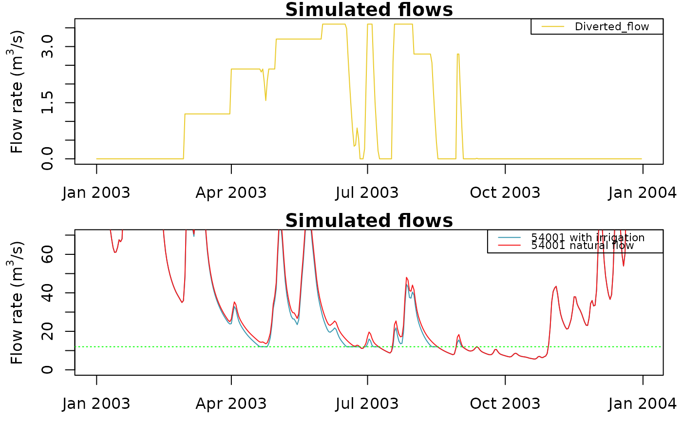
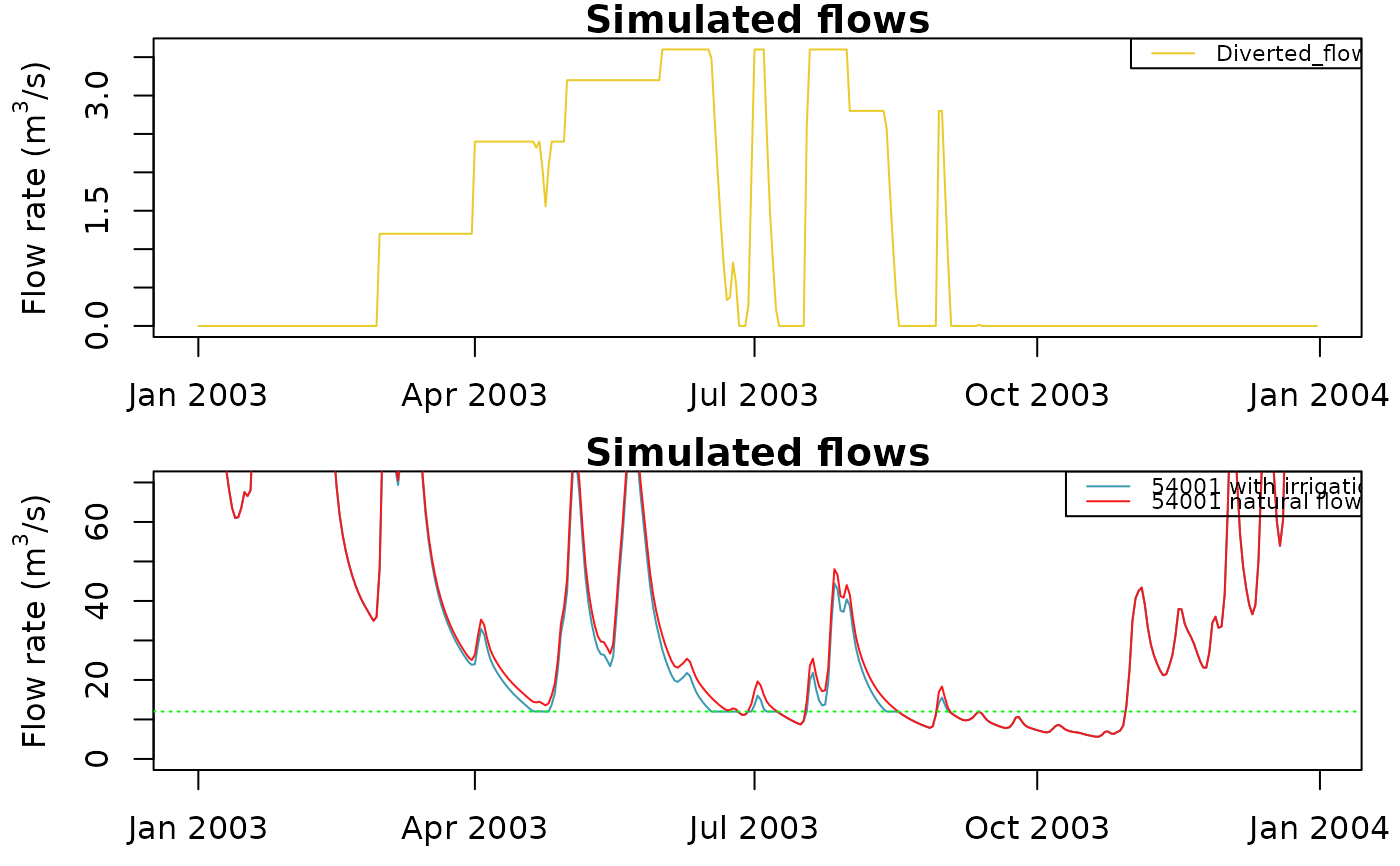
# Retrieve diverted flow at "54001" and convert it from m3/day to m3/s
Qdiv_m3s <- OM_div$`54001`$Qdiv_m3 / 86400
# Plot the diverted flow for the year 2003
Ind_Plot <- which(
OM_div[[1]]$DatesR >= as.POSIXct("2003-01-01", tz = "UTC") &
OM_div[[1]]$DatesR <= as.POSIXct("2003-12-31", tz = "UTC")
)
dfQdiv <- as.Qm3s(DatesR = OM_div[[1]]$DatesR[Ind_Plot],
Diverted_flow = Qdiv_m3s[Ind_Plot])
oldpar <- par(mfrow=c(2,1), mar = c(2.5,4,1,1))
plot(dfQdiv)
# Plot natural and influenced flow at station "54001"
df54001 <- cbind(attr(OM_div, "Qm3s")[Ind_Plot, c("DatesR", "54001")],
attr(OM_severn, "Qm3s")[Ind_Plot, "54001"])
names(df54001) <- c("DatesR", "54001 with irrigation", "54001 natural flow")
df54001 <- as.Qm3s(df54001)
plot(df54001, ylim = c(0,70))
abline(h = 12, col = "green", lty = "dotted")
# }
# Computation of the irrigation withdraw objective
irrigMonthlyPlanning <- c(0.0, 0.0, 1.2, 2.4, 3.2, 3.6, 3.6, 2.8, 1.8, 0.0, 0.0, 0.0)
names(irrigMonthlyPlanning) <- month.abb
irrigMonthlyPlanning
#> Jan Feb Mar Apr May Jun Jul Aug Sep Oct Nov Dec
#> 0.0 0.0 1.2 2.4 3.2 3.6 3.6 2.8 1.8 0.0 0.0 0.0
DatesR_month <- as.numeric(format(DatesR, "%m"))
# Withdrawn flow calculated for each day is negative
Qirrig <- matrix(-irrigMonthlyPlanning[DatesR_month] * 86400, ncol = 1)
colnames(Qirrig) <- "54001"
# Minimum flow to remain downstream the diversion is 12 m3/s
Qmin <- matrix(12 * 86400, nrow = length(DatesR), ncol = 1)
colnames(Qmin) = "54001"
# Creation of GRimwrInputsModel object
IM_div <- CreateInputsModel(g_div, DatesR, Precip, PotEvap, Qinf = Qirrig, Qmin = Qmin)
#> CreateInputsModel.GRiwrm: Processing sub-basin 54095...
#> CreateInputsModel.GRiwrm: Processing sub-basin 54002...
#> CreateInputsModel.GRiwrm: Processing sub-basin 54029...
#> CreateInputsModel.GRiwrm: Processing sub-basin 54001...
#> CreateInputsModel.GRiwrm: Processing sub-basin 54032...
#> CreateInputsModel.GRiwrm: Processing sub-basin 54057...
# RunOptions and parameters are unchanged, we can directly run the simulation
OM_div <- RunModel(IM_div,
RunOptions = RO_severn,
Param = P_severn)
#> RunModel.GRiwrmInputsModel: Processing sub-basin 54095...
#> RunModel.GRiwrmInputsModel: Processing sub-basin 54002...
#> RunModel.GRiwrmInputsModel: Processing sub-basin 54029...
#> RunModel.GRiwrmInputsModel: Processing sub-basin 54001...
#> RunModel.GRiwrmInputsModel: Processing sub-basin 54032...
#> RunModel.GRiwrmInputsModel: Processing sub-basin 54057...
# Retrieve diverted flow at "54001" and convert it from m3/day to m3/s
Qdiv_m3s <- OM_div$`54001`$Qdiv_m3 / 86400
# Plot the diverted flow for the year 2003
Ind_Plot <- which(
OM_div[[1]]$DatesR >= as.POSIXct("2003-01-01", tz = "UTC") &
OM_div[[1]]$DatesR <= as.POSIXct("2003-12-31", tz = "UTC")
)
dfQdiv <- as.Qm3s(DatesR = OM_div[[1]]$DatesR[Ind_Plot],
Diverted_flow = Qdiv_m3s[Ind_Plot])
oldpar <- par(mfrow=c(2,1), mar = c(2.5,4,1,1))
plot(dfQdiv)
# Plot natural and influenced flow at station "54001"
df54001 <- cbind(attr(OM_div, "Qm3s")[Ind_Plot, c("DatesR", "54001")],
attr(OM_severn, "Qm3s")[Ind_Plot, "54001"])
names(df54001) <- c("DatesR", "54001 with irrigation", "54001 natural flow")
df54001 <- as.Qm3s(df54001)
plot(df54001, ylim = c(0,70))
abline(h = 12, col = "green", lty = "dotted")
 par(oldpar)