Performing queries on the 'Ecoulement' API • hubeau

This vignette shows how to use the hubeau R package in order to retrieve data from the French streams drought monitoring network (Observatoire National Des Etiage, ONDE) from the API “Ecoulement des cours d’eau” of the Hub’eau portal.

Nationwide, this network encompasses 3000+ observation sites, that are streams stretches selected to reflect the severity of drought events, i.e. that flow in “normal” conditions but dry out in case of drought. Located at the upstream of the river basins, these sites are expected to act as ‘sentinels’ and to provide early warning of the necessity of restricting water withdrawal in rivers and associated water tables.

We illustrate the use of this API for the departement of Ille-et-Vilaine (code_departement=35) with some example of maps and charts useful for the interpretation of these data.

my_dept <- "35"

Getting started

First, we need to load the packages used in this vignette for processing data and display results on charts and map:

library(hubeau)

library(dplyr)
#> 
#> Attaching package: 'dplyr'
#> The following objects are masked from 'package:stats':
#> 
#>     filter, lag
#> The following objects are masked from 'package:base':
#> 
#>     intersect, setdiff, setequal, union
library(sf)
#> Linking to GEOS 3.10.2, GDAL 3.4.1, PROJ 8.2.1; sf_use_s2() is TRUE
library(mapview)
library(ggplot2)

“Ecoulement” is one of the 11 APIs that can be queried with the hubeau R package. These APIs can be listed using the list_apis() function.

list_apis()
#>  [1] "prelevements"         "indicateurs_services" "hydrometrie"         
#>  [4] "niveaux_nappes"       "poisson"              "ecoulement"          
#>  [7] "hydrobio"             "temperature"          "qualite_eau_potable" 
#> [10] "qualite_nappes"       "qualite_rivieres"

The list of the API endpoints is provided by the function list_endpoints.

list_endpoints(api = "ecoulement")
#> [1] "stations"     "observations" "campagnes"

stations lists the monitoring stations
campagnes lists the surveys
observations is the data itself, indicating if, at the date of the survey, the river flows or if it is dry (which is assessed visually in the field)

station and observations can be joined at least by the field code_station.

observations and campagne can be joined by the field code_campagne.

For each endpoint, the function list_params() gives the different parameters that can be retrieved.

list_params(api = "ecoulement",
            endpoint = "observations")
#>  [1] "format"               "code_station"         "libelle_station"     
#>  [4] "code_departement"     "libelle_departement"  "code_commune"        
#>  [7] "libelle_commune"      "code_region"          "libelle_region"      
#> [10] "code_bassin"          "libelle_bassin"       "code_cours_eau"      
#> [13] "libelle_cours_eau"    "code_campagne"        "code_reseau"         
#> [16] "libelle_reseau"       "date_observation_min" "date_observation_max"
#> [19] "code_ecoulement"      "libelle_ecoulement"   "longitude"           
#> [22] "latitude"             "distance"             "bbox"                
#> [25] "sort"                 "page"                 "size"                
#> [28] "fields"               "Accept"

Retrieving the data

Sites

Retrieve the available fields.

param_stations <- paste(
    list_params(api = "ecoulement", endpoint = "stations"),
    collapse = ","
)

Download the data.

stations <- get_ecoulement_stations(
  code_departement = my_dept,
  fields = param_stations
)

The stations dataframe is transformed into a sf geographical object, then mapped.

stations_geo <- stations %>% 
  select(code_station,
         libelle_station,
         longitude,
         latitude) %>% 
  sf::st_as_sf(coords = c("longitude", "latitude"), crs = 4326)

mapview::mapview(
  stations_geo,
  popup = leafpop::popupTable(
    stations_geo,
    zcol = c("code_station", "libelle_station"),
    feature.id = FALSE,
    row.numbers = FALSE
  ),
  label = "libelle_station", 
  legend = FALSE
)

Surveys

A survey encompasses a series of visual observations carried out on stations at the “departement” grain. It is tagged as “usuelle” if it is a routine (i.e. around the 24th of the month from May to September), as “complémentaire” if not (e.g. during very dry periods).

Download the surveys dataframe.

surveys <- get_ecoulement_campagnes(
  code_departement = my_dept, # department id
  date_campagne_min = "2012-01-01" # start date
  )

surveys <- surveys %>%
  mutate(code_campagne = as.factor(code_campagne), 
         year = lubridate::year(date_campagne),
         month = lubridate::month(date_campagne)) %>%
    select(code_campagne,
           year, 
           month,
           libelle_type_campagne)

Visualise a few rows.

surveys %>%
  head() %>% 
  knitr::kable()

code_campagne	year	month	libelle_type_campagne
96911	2022	10	complémentaire
96868	2022	10	complémentaire
96831	2022	9	usuelle
96724	2022	9	complémentaire
96652	2022	8	usuelle
96562	2022	8	complémentaire

Observations

Retrieve the available fields.

param_obs <- paste(
    list_params(api = "ecoulement", endpoint = "observations"),
    collapse = ","
)

Download the data.

observations <- 
  get_ecoulement_observations(
    code_departement = my_dept,
    date_observation_min = "2012-01-01",
    fields = param_obs
  )

observations <- observations %>%
  filter(!is.na(code_ecoulement)) %>%
  mutate(code_campagne = as.factor(code_campagne))

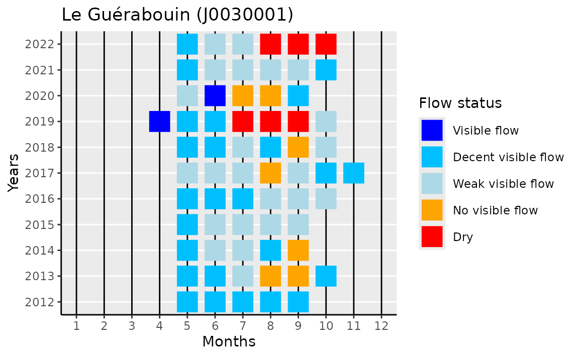
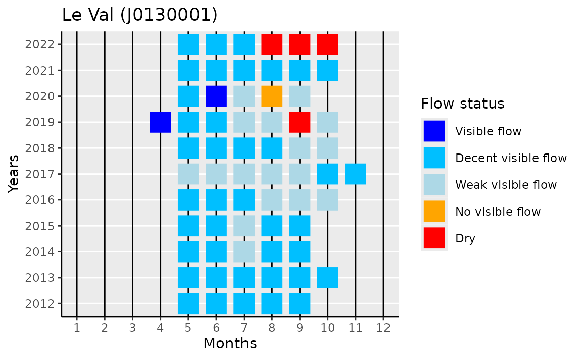
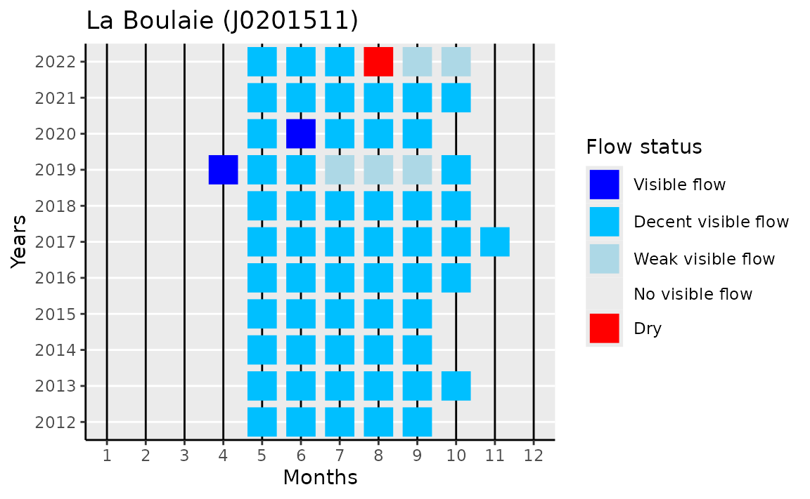
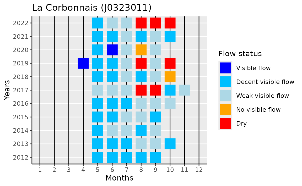
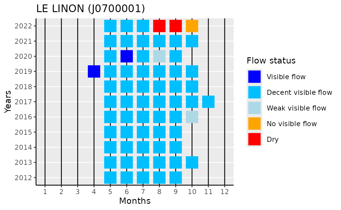
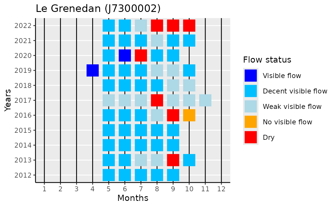
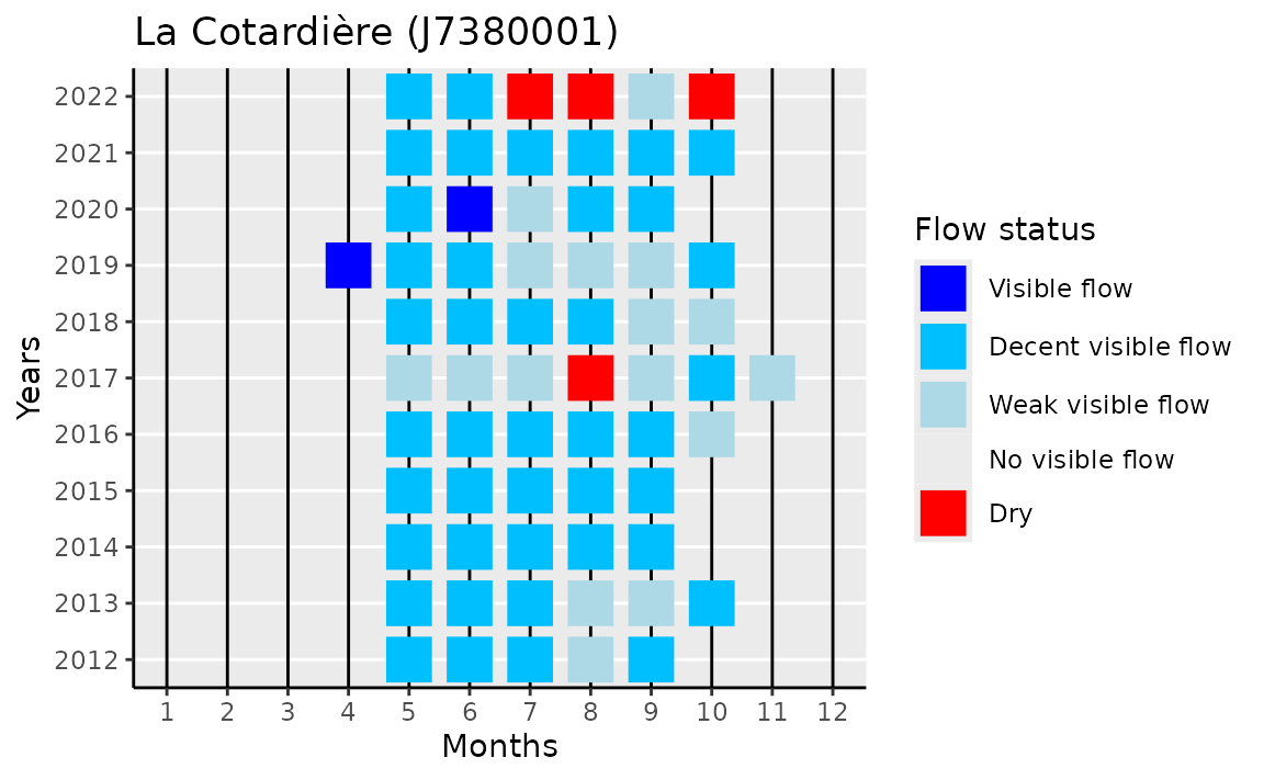
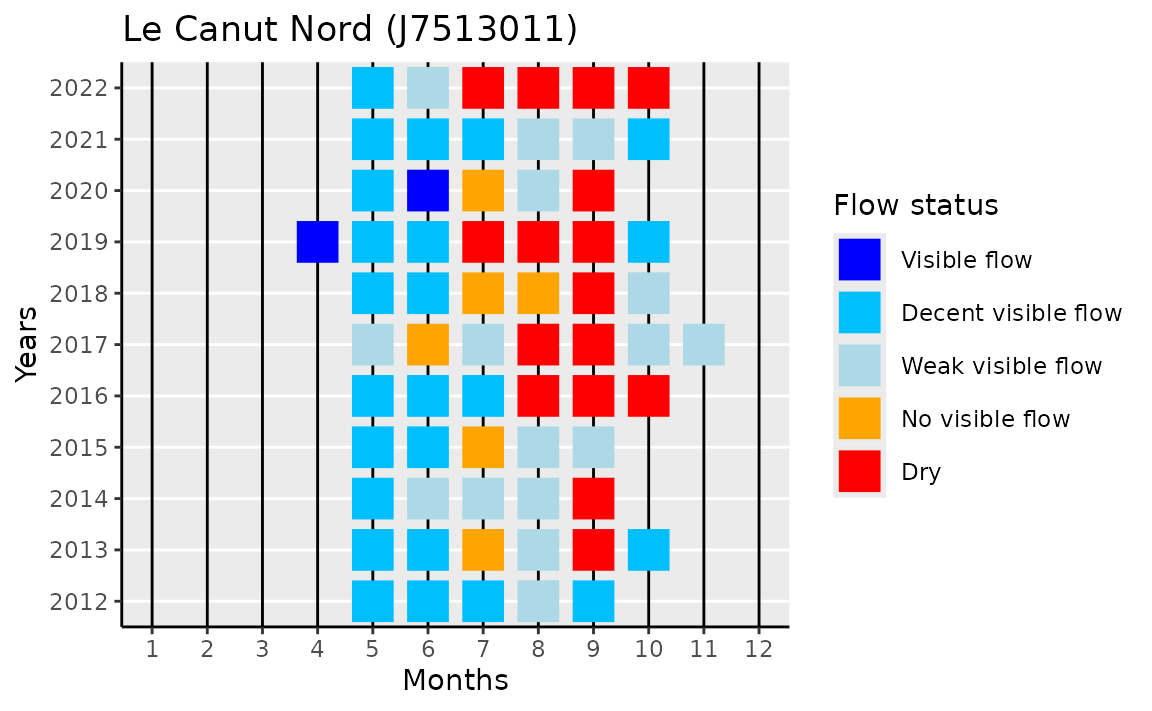
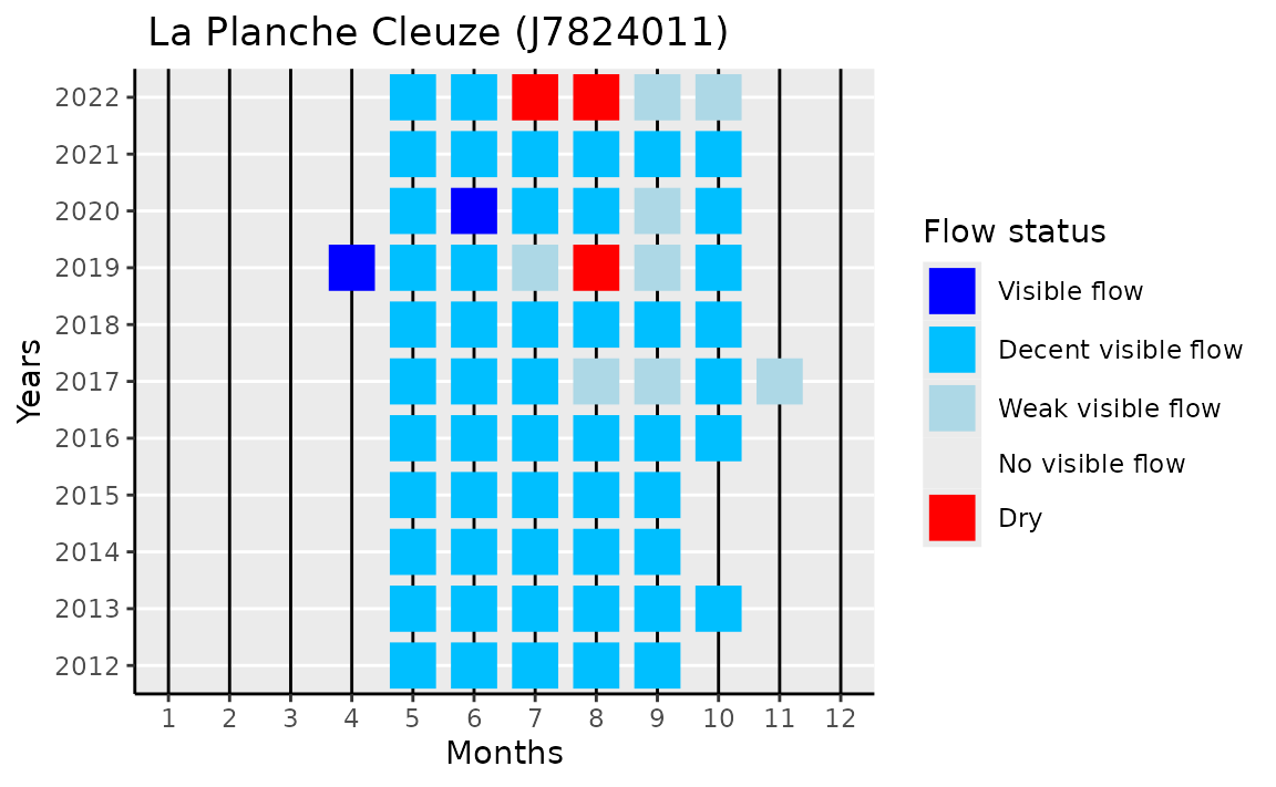
Graphical output of monthly indicator

We first need to join survey and observation data:

obs_and_surv <- observations %>% 
  left_join(surveys, by = join_by(code_campagne)) %>% 
  select(code_station, libelle_station, year, month, code_ecoulement)

And, in case of several observations during the same month, we keep the driest status:

obs_and_surv <- obs_and_surv %>% 
  arrange(code_ecoulement) %>%
  group_by(code_station, libelle_station, year, month) %>%
  summarise(code_ecoulement = last(code_ecoulement), .groups = 'drop')

The flow observations codes are translated in English:

flow_labels <- c(
  "1"  = "Visible flow",
  "1a" = "Decent visible flow",
  "1f" = "Weak visible flow",
  "2"  = "No visible flow",
  "3"  = "Dry"
)
obs_and_surv$flow_label <- flow_labels[obs_and_surv$code_ecoulement]

Custom plot function.

gg_stream_flow <-
  function(sel_station, data) {
    
    # selected data
    sel_data <- data %>%
      filter(code_station == sel_station) %>%
      mutate(flow_label = factor(flow_label, levels = flow_labels))

    # station name for plot title
    station_lab <- unique(sel_data$libelle_station)

    # year range
    year_range <-
      min(sel_data$year, na.rm = T):max(sel_data$year, na.rm = T)
    
    # plot
    sel_data %>%
      ggplot(aes(x = month,
                 y = year,
                 color = flow_label)) +
      geom_point(shape = 15, size = 7) +
      scale_color_manual(name = "Flow status",
                         values = c("blue", 
                                    "deepskyblue", 
                                    "lightblue", 
                                    "orange", 
                                    "red"), 
                         labels = flow_labels, 
                         drop = FALSE) +
      scale_x_continuous(breaks = 1:12,
                         labels = 1:12,
                         limits = c(1, 12)) +
      scale_y_continuous(breaks = year_range,
                         labels = year_range) +
      labs(x = "Months",
           y = "Years",
           title = sprintf("%s (%s)", station_lab, sel_station)) +
      theme(
        axis.line = element_line(color = 'black'),
        plot.background = element_blank(),
        panel.grid.minor = element_blank(),
        panel.grid.major.x = element_line(linewidth = 0.5,
                                          colour = "black"),
        panel.border = element_blank()
      )
  }

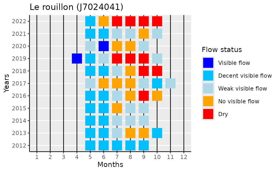
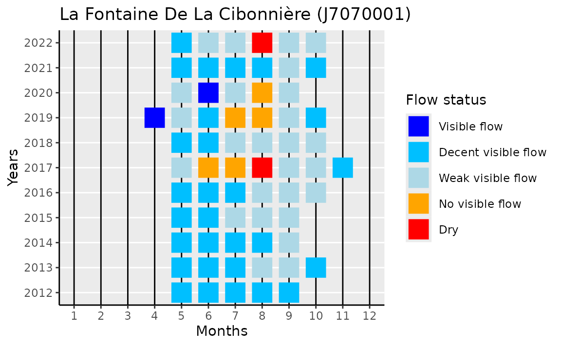
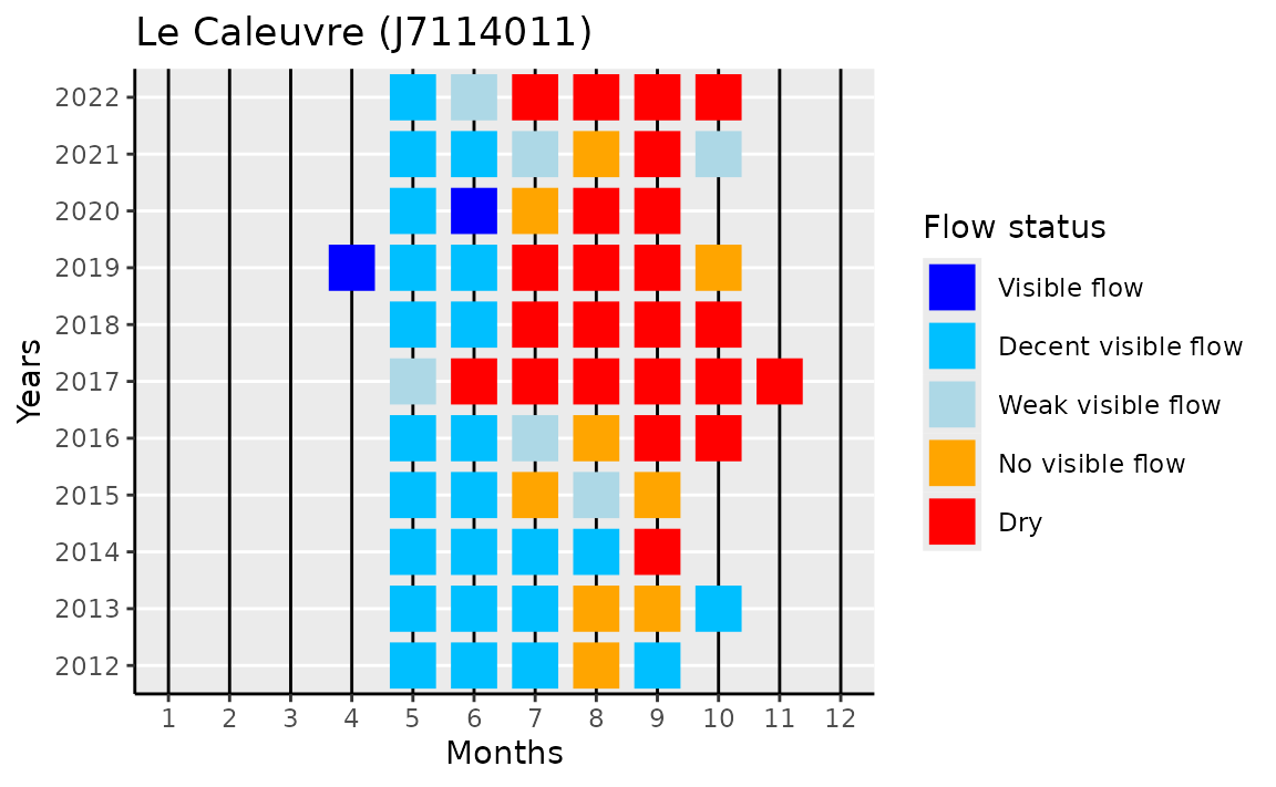
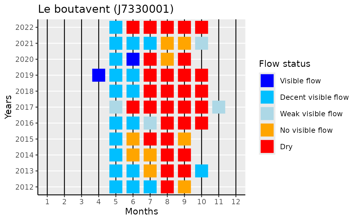
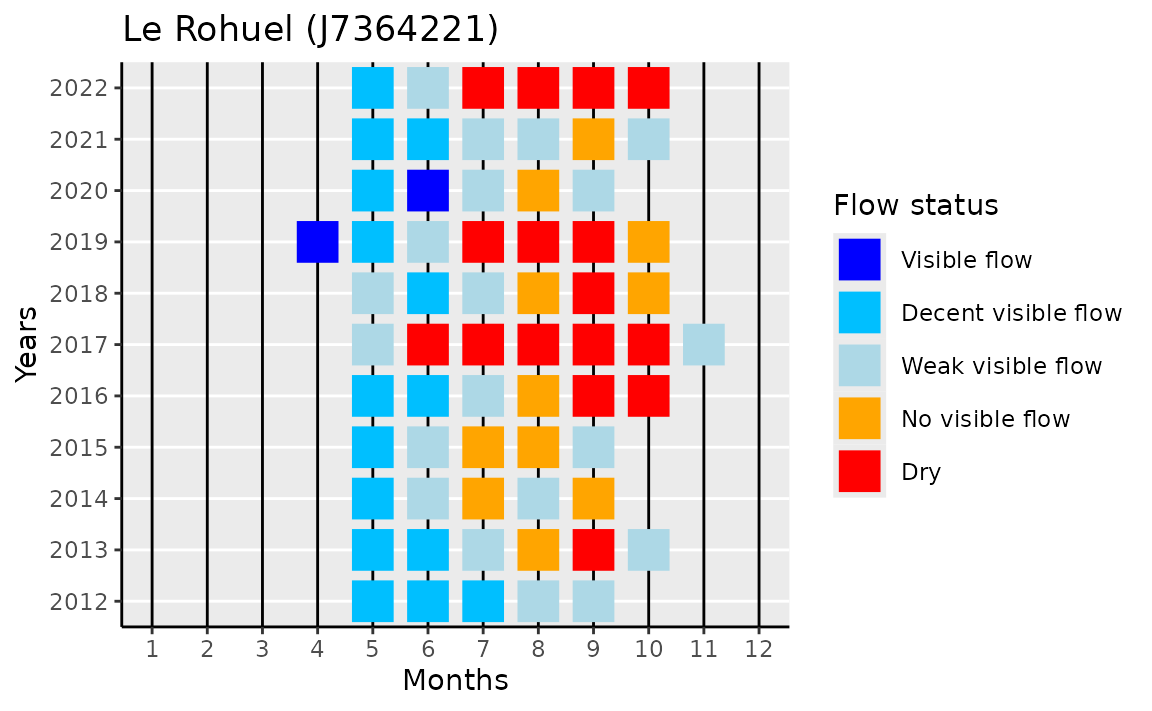
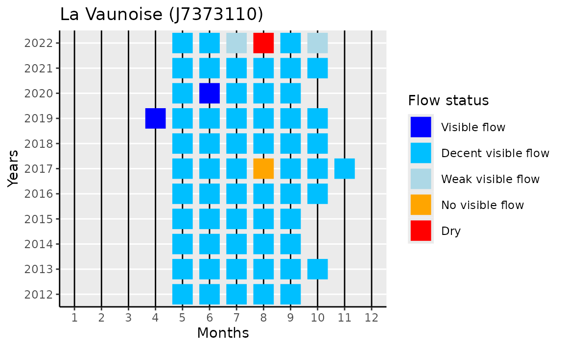
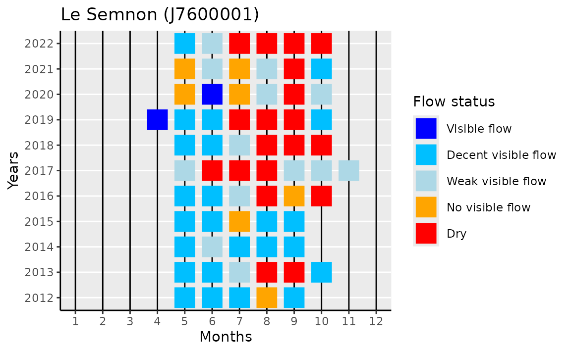
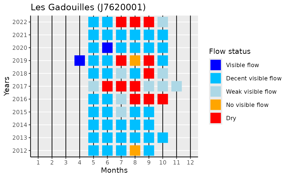
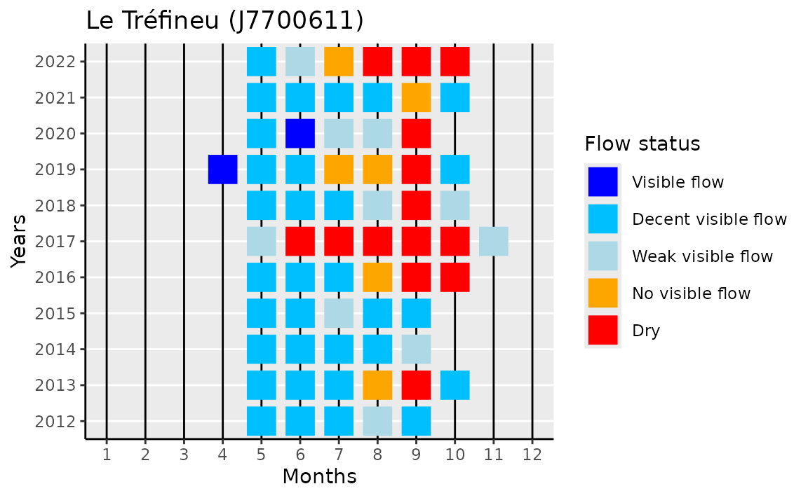
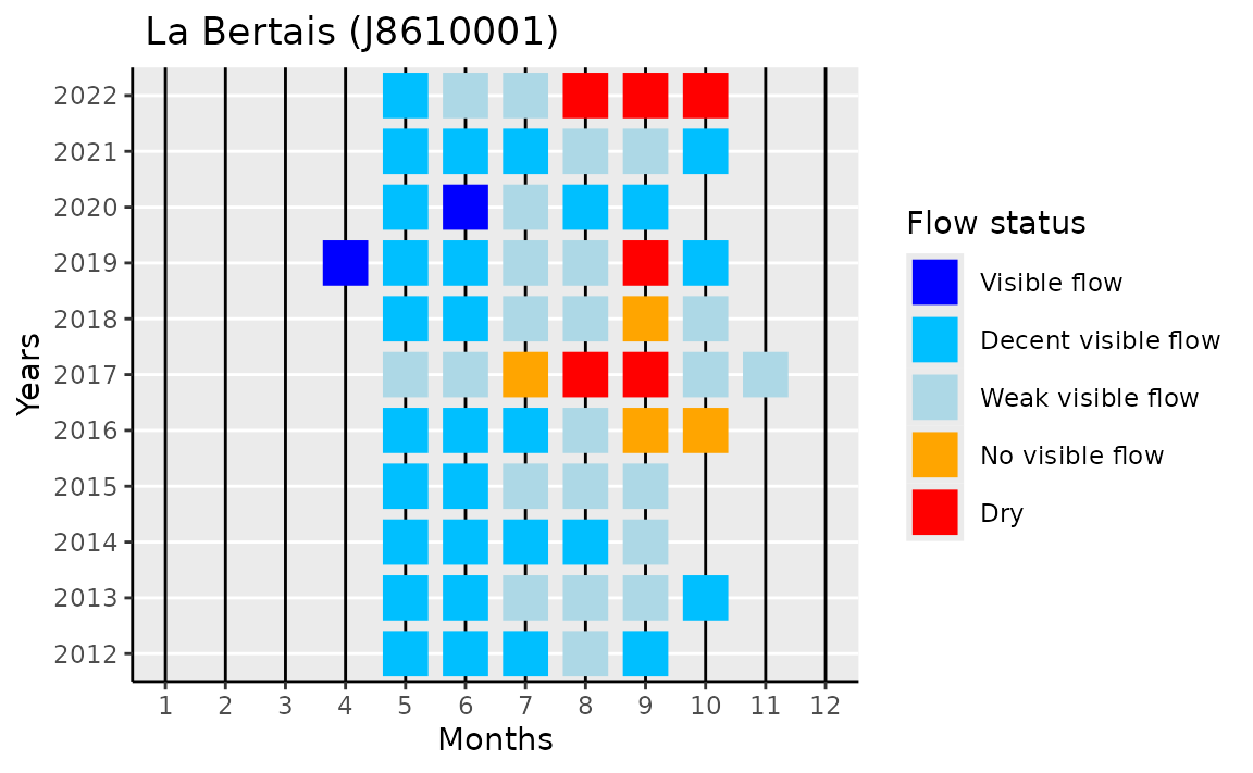
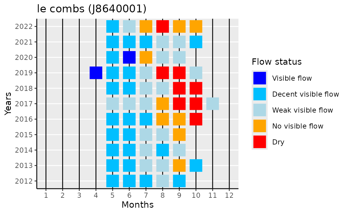
Display plot for all stations that contain at least one observation with “Dry” status.

dry_stations <- obs_and_surv %>% 
  filter(code_ecoulement == "3") %>% 
  pull(code_station) %>% unique

lapply(dry_stations, gg_stream_flow, data = obs_and_surv)

Performing queries on the ‘Ecoulement’ API