Performing queries on the 'niveaux_nappes' API • hubeau

This vignette shows how to use the hubeau R package in order to retrieve data from the French piezometric monitoring network (portail national d’Accès aux Données sur les Eaux Souterraines, ADES) from the API “piézométrie” (or “niveaux nappes”) of the Hub’eau portal.

We illustrate the use of this API for the geological layer “Calcaires et marnes du Dogger du bassin versant du Clain libres” (code=GG063) with an example of map and chart useful for the interpretation of these data.

my_water_table_code <- "GG063"

Getting started

First, we need to load the packages used in this vignette for processing data and display results on charts and map:

library(hubeau)

library(dplyr)
#> 
#> Attaching package: 'dplyr'
#> The following objects are masked from 'package:stats':
#> 
#>     filter, lag
#> The following objects are masked from 'package:base':
#> 
#>     intersect, setdiff, setequal, union
library(sf)
#> Linking to GEOS 3.10.2, GDAL 3.4.1, PROJ 8.2.1; sf_use_s2() is TRUE
library(mapview)
library(ggplot2)
library(purrr)

“niveaux_nappes” is one of the 11 APIs that can be queried with the hubeau R package.

The list of the API endpoints is provided by the function list_endpoints.

list_endpoints(api = "niveaux_nappes")
#> [1] "chroniques"    "chroniques_tr" "stations"

chroniques long-term time series
chroniques_tr real time observations
stations lists the monitoring stations

The tables can be joined at least by the field code_bss (i.e. the site Id).

For each endpoint, the function list_params() gives the different parameters that can be retrieved.

list_params(api = "niveaux_nappes",
            endpoint = "stations")
#>  [1] "bbox"                 "bss_id"               "code_bdlisa"         
#>  [4] "code_bss"             "code_commune"         "code_departement"    
#>  [7] "codes_masse_eau_edl"  "date_recherche"       "fields"              
#> [10] "format"               "nb_mesures_piezo_min" "page"                
#> [13] "size"                 "srid"

Retrieving the data

Sites

Download the data.

stations <- get_niveaux_nappes_stations(
  codes_masse_eau_edl = my_water_table_code
)

Time series

The aim here is to retrieve the time series of water levels measures in the piezometers.

param_chroniques <- paste(
    list_params(api = "niveaux_nappes",
                endpoint = "chroniques"),
    collapse = ","
)

No field allows to select a departement, so it is necessary to iterate through stations.

water_table_level <- map_df(
  .x = stations$code_bss,
  .f = function(x)
    get_niveaux_nappes_chroniques(code_bss = x,
                                  date_debut_mesure = "2015-01-01")
)

Tidying the data

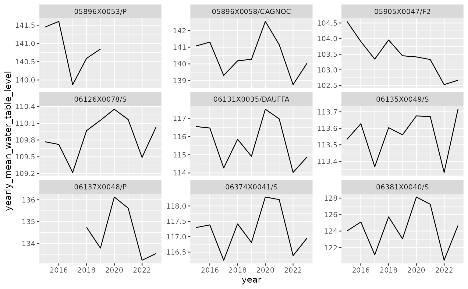
The dataframe is processed to get a ‘year’ and a ‘month’ variables, then averaged by year for each site.

water_table_level <- water_table_level %>% 
  mutate(date_mesure = lubridate::ymd(date_mesure),
         year = lubridate::year(date_mesure),
         month = lubridate::month(date_mesure))

Selection, for each of the stations, of the years with 12 months of data. This is done to prevent incomplete time periods to influence the yearly mean water level excessively.

yearly_mean_water_table_level <- water_table_level %>% 
  group_by(code_bss,
           year) %>% 
    summarise(n_months = n_distinct(month)) %>% 
    filter(n_months == 12) # complete years

yearly_mean_water_table_level <- yearly_mean_water_table_level %>% 
  select(-n_months) %>% 
  left_join(water_table_level) %>% # filtering join
  group_by(code_bss,
           year,
           month) %>% 
    summarise(monthly_mean_water_table_level = mean(niveau_nappe_eau, na.rm = TRUE)) %>% 
  group_by(code_bss,
           year) %>% 
    summarise(yearly_mean_water_table_level = mean(monthly_mean_water_table_level, na.rm = TRUE)) %>% 
  ungroup()

Plotting

ggplot(data = yearly_mean_water_table_level,
       aes(x = year,
           y = yearly_mean_water_table_level)) +
  geom_line() +
  facet_wrap(~code_bss,
             scales = "free_y")

Mapping

The stations data.frame is transformed into a sf geographical object.

stations_geo <- stations %>% 
  st_as_sf(coords = c("x", "y"),
           crs = 4626)

We create a plot for each station ready to be displayed as map “pop-up”.

p <- lapply(unique(yearly_mean_water_table_level$code_bss),
            function(x) {
              ggplot(data = yearly_mean_water_table_level %>% filter(code_bss == x),
                     aes(x = year,
                         y = yearly_mean_water_table_level)) +
                geom_line() +
                labs(title = x)
            })

Then they are mapped using the mapview R package. Click on a spot to popup the plot.

mapview(
  stations_geo,
  map.types = c("OpenStreetMap",
                "Esri.WorldShadedRelief",
                "OpenTopoMap"),
  popup = leafpop::popupGraph(p)
)

Performing queries on the ‘niveaux_nappes’ API

Pascal Irz & David Dorchies